Historical overview
Stage 1: early foundations (1930s–1950s)
Leonid Hurwicz, Jacob Marschak, Trygve Haavelmo, Tjalling Koopmans, and the Cowles Commission
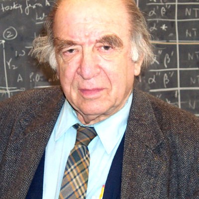
Leonid Hurwicz
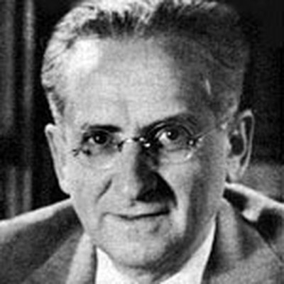
Jacob Marschak
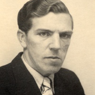
Trygve Haavelmo

Tjalling Koopmans
Key contributions:
Introduced the structural vs reduced form distinction.
Formalized simultaneous equations, endogeneity, identification.
Haavelmo (1944): probability approach to econometrics → modern estimation foundations.
Marschak: structure needed for policy analysis.
Hurwicz: identification theory (order/rank conditions).
Legacy: SEM becomes the dominant approach to causal inference in economics.
Stage 2: the Lucas critique and microfoundations (1970s)
Robert E. Lucas Jr. and the rational expectations revolution

Robert E. Lucas Jr.
Key points:
Structural parameters must be policy invariant.
Ad hoc SEM (with “behavioral equations”) fail under policy changes.
Led to microfounded models derived from optimization and equilibrium conditions.
Birth of DSGE models as dynamic, expectations-driven SEM descendants.
Legacy: SEM concepts survive but become embedded inside microfounded dynamic systems.
Stage 3: individual-level structural modelling (1980s–1990s)
John Rust (1987): dynamic discrete choice V. Joseph Hotz and Robert A. Miller (1993): CCP inversion, reduced-form based identification Steven Berry, James Levinsohn and Ariel Pakes (1995): random-coefficients demand estimation

John Rust

V. Joseph Hotz

Robert A. Miller

Steven Berry

James Levinsohn
Key innovations:
Microfoundations at the agent level (Bellman equations).
Structural estimation using NFXP and GMM.
Discrete choice demand becomes the IO workhorse.
Legacy: structural microeconometrics becomes a major field.
Stage 4: modern structural IO (1990s–2020s)
Richard Ericson and Ariel Pakes (1995) dynamic games Victor Aguirregabiria and Pedro Mira, Ariel Pakes et al., and more recent computational IO

Richard Ericson

Ariel Pakes

Victor Aguirregabiria

Pedro Mira
Advances:
Multi-agent dynamic games, heterogeneous firms, entry/exit, investment.
GMM, simulation, and high-dimensional methods.
Close integration with industrial organization and antitrust practice.
Legacy: modern IO is a fully microfounded, dynamic descendant of SEM.
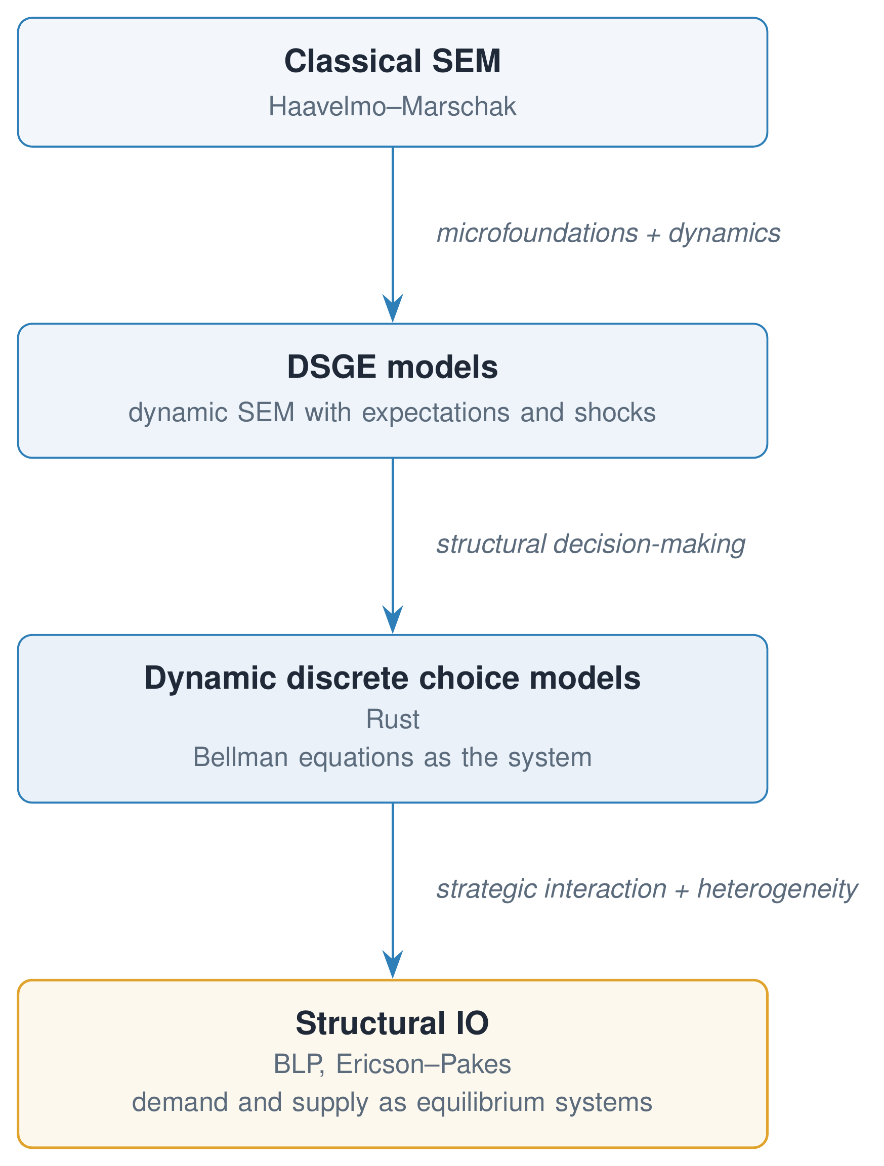
Modern structural econometric models — DSGE, dynamic discrete choice, and structural IO — are dynamic, microfounded generalizations of classical simultaneous equations models (SEM).
Structural and reduced form econometrics
| Aspect | Structural econometrics | Reduced form econometrics |
|---|---|---|
| Essence | Estimation of parameters of economic models derived from theory | Estimation of relationships directly from the data |
| Purpose | Policy analysis, counterfactuals, understanding theoretical mechanisms | Prediction, local causal inference |
| Model | Based on economic theory, optimization behavior | Statistical relationships without explicit economic model |
| Assumptions | About details of economic behavior | About statistical properties of data |
| Identification | Exclusion restrictions, instruments, functional form | Often relies on natural experiments, IV, regression discontinuity |
| Estimation methods | MLE, GMM, simulated methods | OLS, IV, matching, regression discontinuity |
| Data requirements | Often requires detailed microdata | Generally less detailed or aggregate data |
| Applications | Structural models of demand, dynamic programming, games | Reduced form impact evaluations, treatment effects |
Structural econometrics focuses on estimating parameters of economic models derived from theory, allowing for counterfactual analysis and policy simulations.
Reduced form econometrics focuses on estimating relationships directly from data without explicit reference to underlying economic models, often used for prediction or causal inference without structural interpretation.
Is economics a falsifiable science according to Popper (1934)?
How can we estimate the effect of a large new and unique policy?
Can a model be useful without being realistic?
Evidence-based (experimental) vs. model-based (structural) policy analysis -- in medicine?
Why structural econometrics?
Four things a structural approach buys you, each of them a consequence of committing to an explicit model.
Internal consistency. Rational agents facing constraints; uncertainty stated as an explicit probability distribution; well-defined equilibrium concepts (competitive, Nash, and so on); an explicit data-generating process; estimation grounded in the LLN and the CLT.
Elegance and transparency. Every step can be independently verified, and there is little room for researcher discretion — though the numerical implementation can still hide problems.
Causality. A model-based concept of causality, resting on assumptions that are stated rather than implied.
Counterfactuals. Generated by the model itself. They are valid only within the maintained structure, and taking them outside it requires further external validity assumptions.
Components of a structural estimation project
Economic model derived from theory — optimizing agents, possibly with bounded rationality, dynamics, observed and unobserved heterogeneity, and either equilibrium conditions or strategic interaction between agents.
Data generated by that model — cross-section, time series or panel; individual or aggregate; often censored, truncated or incomplete.
Preliminary data analysis — cleaning, descriptive statistics, visualization, and reduced form estimates that feed back into how the model is built.
Estimation method — maximum likelihood (full or limited information), GMM, simulated methods (simulated MLE, method of simulated moments), or Bayesian.
Identification strategy — exclusion restrictions, functional form assumptions, instruments for endogenous variables, policy invariance.
Counterfactual simulations — the estimated model as a synthetic laboratory for welfare effects, market outcomes and policy analysis.
Prototype dynamic discrete choice model
Choices
Periods: , possibly
Actions:
Indicators:
Mutual exclusivity is not restrictive: combinations can be redefined as distinct actions.
States and transitions
Let the state be . This is all the information that is relevant for the decision at time .
Transition probabilities when action is chosen at period
State spaces may be large but are often sparse.
Preferences and expected utility
Flow/current/instantaneous utility at time period when action is chosen
Discount factor
Expected utility
Value functions and Bellman equation
Define the optimal policy as a vector of zeros and one, indicating the most desirable action.
The value function conditions on optimal behavior in all future periods; it is the maximal attainable expected utility from period on
Bellman equation:
We will see later how the Bellman equation can be solved and value functions computed numerically.
Define the choice-specific value:
By definition the optimal choice is:
Why unobserved heterogeneity is needed
If agents with identical observed states are observed in the data to choose differently
the model implies indifference between actions
all actions appear optimal
the model loses empirical content!
Therefore fully observed heterogeneity is useless for data analysis.
Unobserved heterogeneity framework
Decompose the state:
: observed by both agents and econometrician
: unobserved by econometrician, but observed by agents
The objective becomes predicting choice probabilities, not individual choices.
Data generating process
Observed data are states and corresponding choices:
with the individual observations given by
The likelihood integrates out unobservables:
A huge multidimensional integral in the general case!
We will see how Rust’s assumptions simplify this drastically
Maximum likelihood estimation
Let index utilities, transitions, and .
Early applications include Miller (1984) and Wolpin (1984).
Other estimation approaches:
Two-step methods based on conditional choice probabilities estimated directly from the data (CCP methods) (Hotz–Miller, Aguirregabiria–Mira)
Method of simulated moments (MSM)
Calibration (no standard errors)
Multiple decision makers equilibrium models
Macro style models with aggregate states
Infinitely many agents
Individual actions do not affect aggregate states
Aggregate states affect individual payoffs and transitions
Aggregate states evolve according to the collective behavior of all agents
Dynamic Markov games
Finite number of agents
Individual actions affect payoffs and transitions of all other agents
Joint individual actions affect payoffs and transitions
Equilibrium defined by mutual best responses
Nash
Bayesian Nash
Markov perfect equilibrium (MPE)
Oblivious equilibrium, etc.
- Gillingham, K., Iskhakov, F., Munk-Nielsen, A., Rust, J., & Schjerning, B. (2022). Equilibrium Trade in Automobiles. Journal of Political Economy, 130(10), 2534–2593. 10.1086/720463
- Keane, M. (2010). Structural vs. atheoretic approaches to econometrics. Journal of Econometrics, 156(1), 3–20. https://econpapers.repec.org/article/eeeeconom/v_3a156_3ay_3a2010_3ai_3a1_3ap_3a3-20.htm
- Wolpin, K. I. (2013). The Limits of Inference without Theory. The MIT Press. 10.7551/mitpress/9258.001.0001
- Rust, J. (2014). The Limits of Inference with Theory: A Review of Wolpin (2013). Journal of Economic Literature, 52(3), 820–850. 10.1257/jel.52.3.820
- Sargent, T. J. (2024). Critique and consequence. Journal of Monetary Economics, 141, 2–13. 10.1016/j.jmoneco.2023.10.001