Two classic algorithms for solving , either as an equation or system of equations, or as FOC of an optimization problem. These will be referred to in this course a countless number of times.
Running the code for this lecture
Every code example below is also a runnable notebook in the course code repository,
in the folder session05-sep8/.
You should have cloned that repository already — if not, the instructions are in the algorithms and complexity lecture.
Update your copy before the class. Editing a file in place makes git pull refuse to
update it, so discard whatever you changed while experimenting:
cd sb-dse-code
git reset --hard HEAD
git pull
Nothing in this repository is submitted, so experiment freely — but copy anything you want to keep out of it first, or commit that to a branch of your own.
Setting up the Python environment is covered in Python.
Homework delta_newton_fractals: Newton fractals
Graded homework: task delta_newton_fractals in the class repository. Collect it and work on a
copy in your own repository:
git pull upstream main                                             # collect the task
cp -r tasks/delta_newton_fractals solutions/delta_newton_fractals  # work on the copy
Map the basins of attraction of Newton’s method on the function of this chapter: run the solver from a grid of starting points and color each one by the critical point it reaches. Two versions, side by side — plain Newton, and Newton with the step-halving line search.
The notebook newton_fractals.ipynb in the task folder carries with its gradient
and Hessian, and the same map worked out for the cubic of the first example, which is
the picture to replicate. The code of this class, session05-sep8/ in the code
repository, is worth having beside you while you work.
Submit it as a pull request, following the git workflow. The solutions are discussed at the start of the next class.
Bisection method
Consider first the one-dimensional equations of the form
The latter condition requires that the function takes different signs at the endpoints and .
The algorithm is similar to binary search, but in continuous space.
Input: function f(x)
       brackets [a,b] such that f(a)f(b)<0
       convergence tolerance epsilon
       maximum number of iterations max_iter

Algorithm:
  step 0: ensure all conditions are satisfied
  step 1: compute the sign of the function at (a+b)/2
  step 2: replace a with (a+b)/2 if f(a)f((a+b)/2)>0, otherwise replace b with (a+b)/2
  step 3: repeat steps 1-2 until |a-b| < epsilon, or max_iter number of iterations is reached
  step 4: return (a+b)/2
def bisection(f,a=0,b=1,tol=1e-6,maxiter=100,callback=None):
'''Bisection method for solving equation f(x)=0
on the interval [a,b], with given tolerance and number of iterations.
Callback function is invoked at each iteration if given.
'''
if f(a)*f(b)>0:
raise ValueError('Function has the same sign at the bounds')
for i in range(maxiter):
err = abs(b-a)
if err<tol: break
x = (a+b)/2
if callback != None: callback(err=err,x=x,iter=i,a=a,b=b)
a,b = (x,b) if f(a)*f(x)>0 else (a,x)
else:
raise RuntimeError('Failed to converge in %d iterations'%maxiter)
return xSource
import numpy as np
import matplotlib.pyplot as plt
plt.rcParams['figure.figsize'] = [9, 6]

f = lambda x: -4*x**3+5*x+1
a,b = -3,-.5  # upper and lower limits
xd = np.linspace(a,b,1000)  # x grid
ylim = [-5,25]  # vertical zoom: what matters is the sign, the function runs off the top
def plot_step(a,b,x,iter,**kwargs):
    plot_step.counter += 1
    if iter<7:
        lo,hi = (x,b) if f(a)*f(x)>0 else (a,x)  # the half that is kept
        plt.plot(xd,f(xd),c='red')  # plot the function
        plt.plot([xd[0],xd[-1]],[0,0],c='black')  # plot zero line
        plt.fill_between([a,b],*ylim,color='grey',alpha=0.10)  # current bracket
        plt.fill_between([lo,hi],*ylim,color='green',alpha=0.15)  # the half to keep
        plt.plot([a,a],ylim,c='grey')  # plot lower bound
        plt.plot([b,b],ylim,c='grey')  # plot upper bound
        plt.plot([x,x],ylim,c='green')  # plot the midpoint
        plt.scatter([a,b,x],[f(a),f(b),f(x)],c=['grey','grey','green'],zorder=3)
        plt.title('Iteration %d: [%1.4f,%1.4f], f(x)=%+1.4f, keep [%1.4f,%1.4f]'
                  %(iter+1,a,b,f(x),lo,hi))
        plt.xlim(xd[0],xd[-1])
        plt.ylim(ylim)
        plt.show()
plot_step.counter = 0  # new public attribute
bisection(f,a,b,callback=plot_step)
print('Converged in %d steps'%plot_step.counter)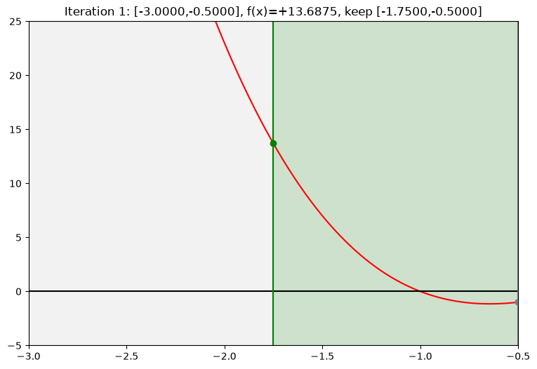
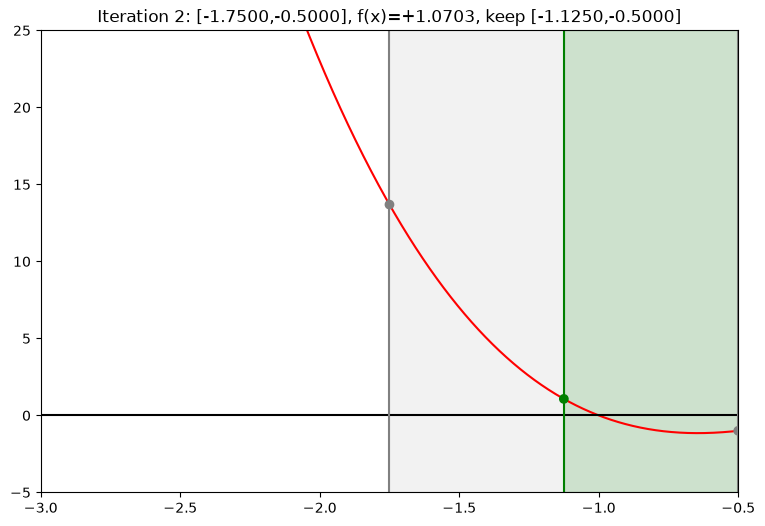
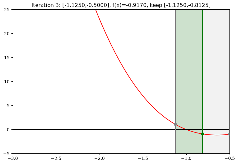
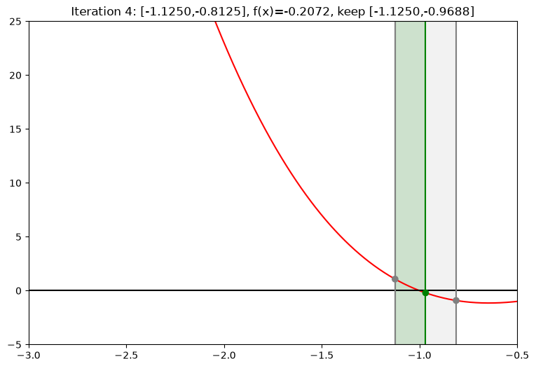
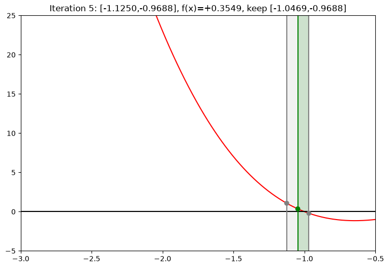
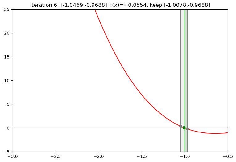
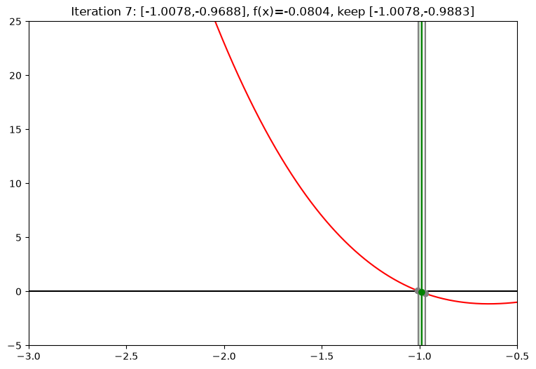
Converged in 22 steps
Bisection is slow but bulletproof: given a valid bracket it always converges, at a linear rate, halving the interval each step.
Remember this when we get to solving complex models — a robust but slow method makes an excellent fallback in the complex problems.
Newton–Raphson method
The second of the two classic solution methods; this one is gradient based.
General form
Equation solving
Finding a maximum/minimum based on the FOC, in which case
System of equations , ,
Derivation of Newton step
Remember the Taylor series expansion
Take the first two terms around the solution , and let and (step towards the solution)
The main idea of the Newton–Raphson method is to iterate on this equation starting from some
It is applicable to systems of equations, in which case and , with the derivative replaced by the Jacobian.
Input: function f(x)
       gradient function f'(x)
Algorithm:
1. Start with some good initial value
2. Update x using the Newton step above
3. Iterate until convergence
def newton(fun,grad,x0,tol=1e-6,maxiter=100,callback=None):
'''Newton method for solving equation f(x)=0
with given tolerance and number of iterations.
Callback function is invoked at each iteration if given.
'''
for i in range(maxiter):
x1 = x0 - fun(x0)/grad(x0)
err = abs(x1-x0)
if callback != None: callback(err=err,x0=x0,x1=x1,iter=i)
if err<tol: break
x0 = x1
else:
raise RuntimeError('Failed to converge in %d iterations'%maxiter)
return (x0+x1)/2Source
f = lambda x: -4*x**3+5*x+1
g = lambda x: -12*x**2+5
a,b = -3,-.5  # upper and lower limits
xd = np.linspace(a,b,1000)  # x grid
def plot_step(x0,x1,iter,**kwargs):
    plot_step.counter += 1
    if iter<5:
        plt.plot(xd,f(xd),c='red')  # plot the function
        plt.plot([a,b],[0,0],c='black')  # plot zero line
        ylim = [min(f(b),0),f(a)]
        plt.plot([x0,x0],ylim,c='grey') # plot x0
        l = lambda z: g(x0)*(z - x1)
        plt.plot(xd,l(xd),c='green')  # plot the tangent line
        plt.ylim(bottom=10*f(b))
        plt.title('Iteration %d'%(iter+1))
        plt.show()
plot_step.counter = 0  # new public attribute
newton(f,g,x0=-2.5,callback=plot_step)
print('Converged in %d steps'%plot_step.counter)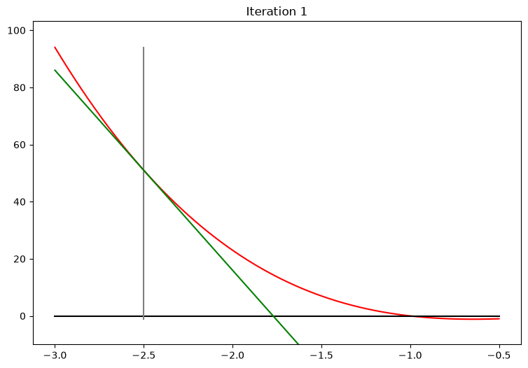
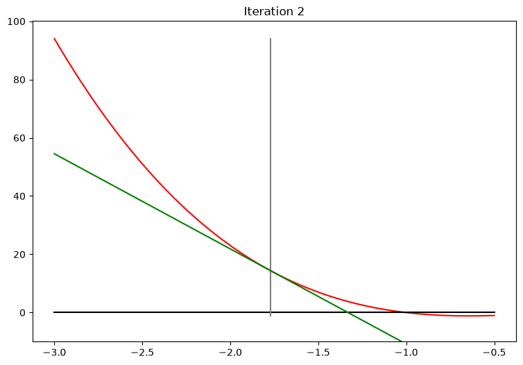
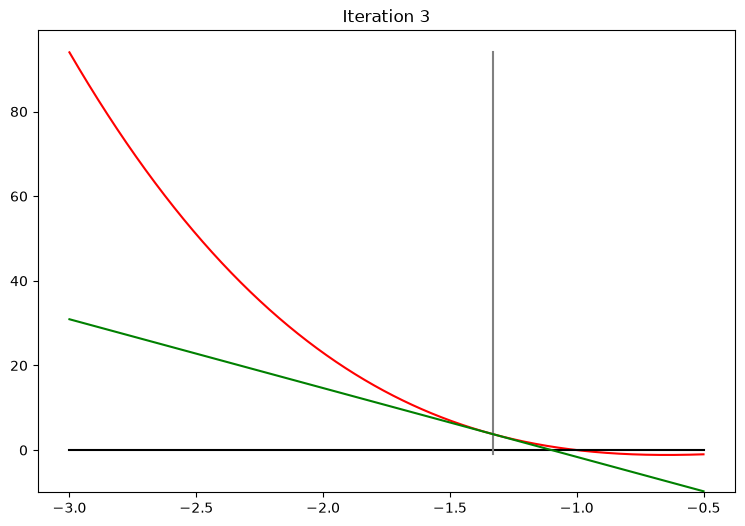
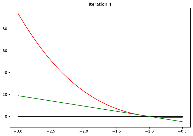
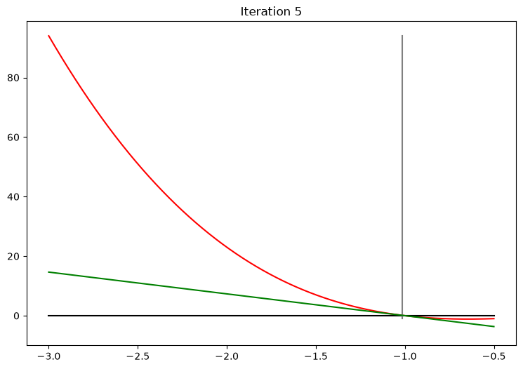
Converged in 7 steps
Rates of convergence and complexity
Which of the two algorithms is intuitively faster?
Fundamentally why?
Continue the example above with a different callback function to print the errors at each iteration.
Source
xstar = -1.0  # f(-1) = 4-5+1 = 0, the exact root in the bracket

def print_err(iter,err,**kwargs):
    '''Report the error at each iteration of either solver.
    Bisection passes the midpoint as x, Newton–Raphson the new point as x1.
    '''
    x = kwargs['x'] if 'x' in kwargs else kwargs['x1']
    print('%3d:  x = %+1.14f   |x-x*| = %1.3e   reported err = %1.3e'
          %(iter,x,abs(x-xstar),err))

print('Bisection on [-3,-0.5]')
bisection(f,-3,-.5,callback=print_err)
print('\nNewton–Raphson from x0=-2.5')
newton(f,g,x0=-2.5,callback=print_err)
Bisection on [-3,-0.5]
0: x = -1.75000000000000 |x-x*| = 7.500e-01 reported err = 2.500e+00
1: x = -1.12500000000000 |x-x*| = 1.250e-01 reported err = 1.250e+00
2: x = -0.81250000000000 |x-x*| = 1.875e-01 reported err = 6.250e-01
3: x = -0.96875000000000 |x-x*| = 3.125e-02 reported err = 3.125e-01
4: x = -1.04687500000000 |x-x*| = 4.688e-02 reported err = 1.562e-01
5: x = -1.00781250000000 |x-x*| = 7.812e-03 reported err = 7.812e-02
6: x = -0.98828125000000 |x-x*| = 1.172e-02 reported err = 3.906e-02
7: x = -0.99804687500000 |x-x*| = 1.953e-03 reported err = 1.953e-02
8: x = -1.00292968750000 |x-x*| = 2.930e-03 reported err = 9.766e-03
9: x = -1.00048828125000 |x-x*| = 4.883e-04 reported err = 4.883e-03
10: x = -0.99926757812500 |x-x*| = 7.324e-04 reported err = 2.441e-03
11: x = -0.99987792968750 |x-x*| = 1.221e-04 reported err = 1.221e-03
12: x = -1.00018310546875 |x-x*| = 1.831e-04 reported err = 6.104e-04
13: x = -1.00003051757812 |x-x*| = 3.052e-05 reported err = 3.052e-04
14: x = -0.99995422363281 |x-x*| = 4.578e-05 reported err = 1.526e-04
15: x = -0.99999237060547 |x-x*| = 7.629e-06 reported err = 7.629e-05
16: x = -1.00001144409180 |x-x*| = 1.144e-05 reported err = 3.815e-05
17: x = -1.00000190734863 |x-x*| = 1.907e-06 reported err = 1.907e-05
18: x = -0.99999713897705 |x-x*| = 2.861e-06 reported err = 9.537e-06
19: x = -0.99999952316284 |x-x*| = 4.768e-07 reported err = 4.768e-06
20: x = -1.00000071525574 |x-x*| = 7.153e-07 reported err = 2.384e-06
21: x = -1.00000011920929 |x-x*| = 1.192e-07 reported err = 1.192e-06
Newton–Raphson from x0=-2.5
0: x = -1.77142857142857 |x-x*| = 7.714e-01 reported err = 7.286e-01
1: x = -1.33114944950557 |x-x*| = 3.311e-01 reported err = 4.403e-01
2: x = -1.09877514383983 |x-x*| = 9.878e-02 reported err = 2.324e-01
3: x = -1.01315263007170 |x-x*| = 1.315e-02 reported err = 8.562e-02
4: x = -1.00028616796687 |x-x*| = 2.862e-04 reported err = 1.287e-02
5: x = -1.00000014027560 |x-x*| = 1.403e-07 reported err = 2.860e-04
6: x = -1.00000000000003 |x-x*| = 3.375e-14 reported err = 1.403e-07
-1.000000070137816Two things stand out:
bisection needs 22 iterations where Newton needs 7!
unlike Newton, the error of bisection is not monotone: it grows at every second step, because the midpoint of a bracket can easily sit further from the root than the previous midpoint did. What halves exactly, every single time, is the bracket, and that is what the solver reports as
err.
The same callback mechanism, now storing and plotting the errors instead of printing them, gives the picture:
Source
def collect(store):
    '''Make a callback that appends (true error, reported error) to the given list'''
    def cb(iter,err,**kwargs):
        x = kwargs['x'] if 'x' in kwargs else kwargs['x1']
        store.append((abs(x-xstar),err))
    return cb

eb, en = [], []
bisection(f,-3,-.5,callback=collect(eb))
newton(f,g,x0=-2.5,callback=collect(en))
eb, en = np.array(eb), np.array(en)

plt.semilogy(np.arange(1,len(eb)+1),eb[:,0],'o',c='blue',label=r'bisection $|x_k-x^\star|$')
plt.semilogy(np.arange(1,len(eb)+1),eb[:,1],'-',c='blue',alpha=.5,label='bisection bracket width')
plt.semilogy(np.arange(1,len(en)+1),en[:,0],'o-',c='red',label=r'Newton–Raphson $|x_k-x^\star|$')
plt.xlabel('iteration $k$')
plt.legend()
plt.grid(True,which='both',alpha=.3)
plt.show()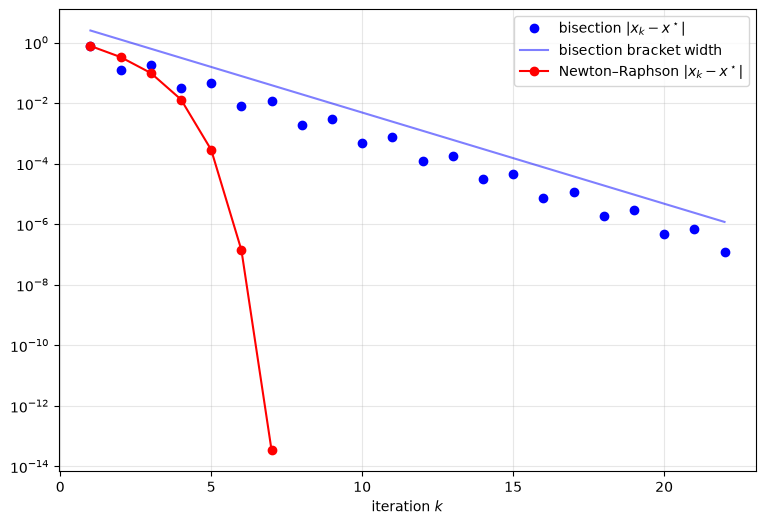
On a log scale linear convergence is a straight line — the error is multiplied by the same factor every iteration.
Quadratic convergence is a cliff: the number of correct digits doubles, so the curve bends down without limit until it hits machine precision.
Bisection took 22 iterations and Newton 7. Is that the right way to compare them?
The Newton curve stops at 10-14 and cannot go lower. Why?
Algorithmic complexity
Let’s take a loot at the algorithmic complexity of the two methods now.
What is the size of the problem for the solvers?
Given the importance of the the desired precision of the solution, the rate of convergence is therefore part of the computational complexity of the algorithm, and the two questions to ask of each method are how many iterations it needs to reach a given accuracy, and what one iteration costs.
Suppose we want to find a root of to accuracy .
Bisection: one binary digit per iteration
Starting from an interval of width , each iteration halves the interval, so after steps the error is bounded by
To achieve we need , that is
Each iteration gains approximately one binary digit of accuracy, whatever the function looks like. That is the flip side of being bulletproof: the bound holds always, and it is never beaten.
Newton–Raphson: doubling the number of digits
Under certain regularity conditions the error of the Newton iteration satisfies
where constant depends on the and .
The number of correct digits approximately doubles with each iteration.
Schematically , and to obtain we need , hence
Counted in digits rather than in , the same statement reads: calculating a root of with -digit precision, provided that a good initial approximation is known, costs , where is the cost of calculating with -digit precision. Both the number of iterations and the price of a single iteration grow with the precision demanded.
Note the words locally and provided that a good initial approximation is known. Everything in this subsection is conditional on being close enough to the root!
Multivariate Newton: the cost of one iteration
In dimensions, for , the Newton step is no longer a division but the solution of a linear system
For a dense Hessian that costs per iteration, so once the iterations are in the region of quadratic convergence the overall cost is roughly
The iteration count barely depends on the accuracy we ask for; the dimension of the problem is what hurts. This is why the structure of the Jacobian matters so much in practice — sparsity, block structure, or an analytical inverse turn the into something affordable.
| Method | Convergence | Iterations for accuracy | Cost per iteration |
|---|---|---|---|
| Bisection | linear | one evaluation of | |
| Newton–Raphson | quadratic, locally | one evaluation of and , up to |
The key distinction between the two methods is therefore:
Bisection — cheap iterations, linear convergence, no way to fail
Newton — expensive iterations, quadratic local convergence, and no guarantee of getting there at all
Can we get the best of the both approaches? How?
When does Newton–Raphson fail?
Newton–Raphson is fast but fragile: quadratic convergence near the root, but what happens away from the root?
Five things can go wrong, in rough order of how often they bite in economic applications:
Multiple solutions — the method converges, but to a root you did not want
Divergence — the iterations run away, or converge to a root far outside the region of interest: the domain of attraction problem
Cycles — the iterations enter a loop and never converge
Function domain and differentiability — a Newton step leaves the region where or is defined
Reduced performance — quadratic convergence is lost in special cases
Multiple solutions
The function of the first example has three roots.
Which one Newton returns is decided by the starting value alone, and the mapping from starting values to roots is neither monotone nor otherwise well behaved.
Starting Newton-Raphson from
Source
def newton_pic(f,g,x0,a=0,b=1,**kwargs):
    '''Illustrate the Newton method iterations on the interval [a,b]'''
    xd = np.linspace(a,b,1000)
    plt.plot(xd,f(xd),c='red')       # the function
    plt.plot([a,b],[0,0],c='black')  # zero line
    def plot_step(**kw):
        plot_step.counter += 1
        z0,z1 = kw['x0'],kw['x1']
        plt.plot([z0,z0],[0,f(z0)],c='green')  # from the axis up to the function
        plt.plot([z0,z1],[f(z0),0],c='green')  # tangent line down to the axis
    plot_step.counter = 0
    try:
        xs = newton(f,g,x0,callback=plot_step,**kwargs)
        plt.title('Started at %1.3f, converged to %1.5f in %d steps'%(x0,xs,plot_step.counter))
    except RuntimeError:
        plt.title('Started at %1.3f, failed to converge in %d iterations'%(x0,plot_step.counter))
    plt.xlim((a,b))
    plt.show()

f = lambda x: -4*x**3+5*x+1  # function
g = lambda x: -12*x**2+5     # derivative
for x0 in [-0.565,-0.58,-0.595]:
    newton_pic(f,g,x0,a=-3,b=1.5)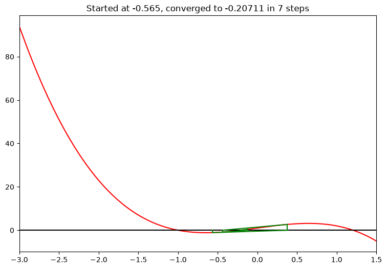
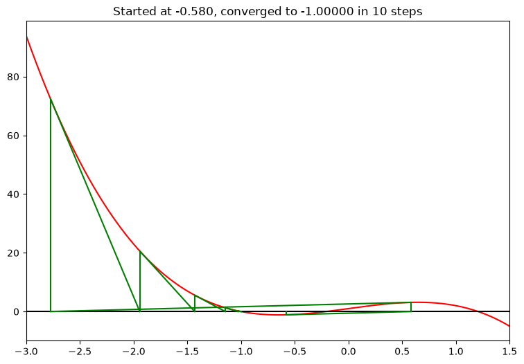
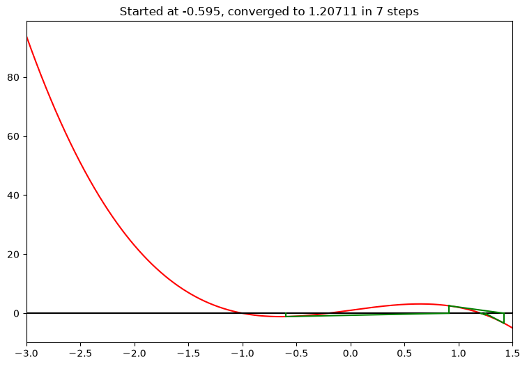
Be aware is all that can be said here: multiple roots are a property of the problem, not of the algorithm.
In structural work this is the situation where the same solver, started from different points, produces different estimates.
Divergence and the domain of attraction
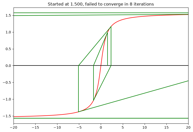
has a single root at , and Newton still fails from a starting point that is only slightly too far out: the tangent overshoots, and each step overshoots by more than the last.
Starting values
Source
f = lambda x: np.arctan(x)
g = lambda x: 1/(1+x**2)
newton_pic(f,g,x0=1.25,a=-20,b=20)            # inside the domain of attraction
newton_pic(f,g,x0=1.5,a=-20,b=20,maxiter=8)   # outside it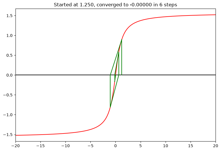
Cycles
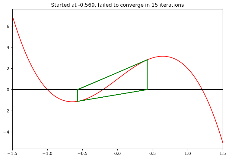
The iterations can also enter a cycle, returning to the same point every second step.
In the example below I had to compute the appropriate starting value numerically (using Newton method to the equation “two Newton steps return me where I started”), but this can happen in practice due to analytical properties of the function being solved. Important to be aware of such possibility.
Source
f = lambda x: -4*x**3+5*x+1  # function
g = lambda x: -12*x**2+5     # derivative
h = lambda x: -24*x          # second derivative

ns = lambda x: x - f(x)/g(x)          # the Newton step itself
ds = lambda x: f(x)*h(x)/g(x)**2      # its derivative
f2 = lambda x: ns(ns(x)) - x          # two Newton steps return to the start
g2 = lambda x: ds(ns(x))*ds(x) - 1    # derivative of the above

x0 = newton(f2,g2,x0=-0.56,tol=1e-16)  # find the cycling starting point
print('To cycle start with x0 = %1.16f'%x0)

newton_pic(f,g,x0,a=-1.5,b=1.5,maxiter=15)
To cycle start with x0 = -0.5689842546416416
Function domain and differentiability
Nothing in the Newton step knows where is defined. Solving from
, the very first step lands on a negative number and every value after that
is nan.
Source
f = lambda x: np.log(x)
g = lambda x: 1/x
newton_pic(f,g,x0=2.9,a=0.001,b=3)
/tmp/ipykernel_3879/2475852609.py:1: RuntimeWarning: invalid value encountered in log
f = lambda x: np.log(x)
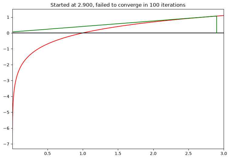
This is the failure mode to expect in many structural models.
The usual remedies are reparametrization (solve in rather than ) or specialized algorithms.
Suboptimal performance
Quadratic convergence requires a simple root, . At a root of multiplicity the method still converges, but only linearly, at rate . For that is : a hundred iterations to reach the tolerance that the first example reached in seven.
Source
f = lambda x: x**9   # a very special case: root of multiplicity 9
g = lambda x: 9*x**8
newton_pic(f,g,x0=1.0,a=-1.5,b=1.5)

def print_err(**kwargs):
    if kwargs['iter'] % 5 == 0:
        print('{:4d}:  x = {:17.14f}  err = {:8.6e}'.format(kwargs['iter'],kwargs['x1'],kwargs['err']))
newton(f,g,x0=1.0,callback=print_err)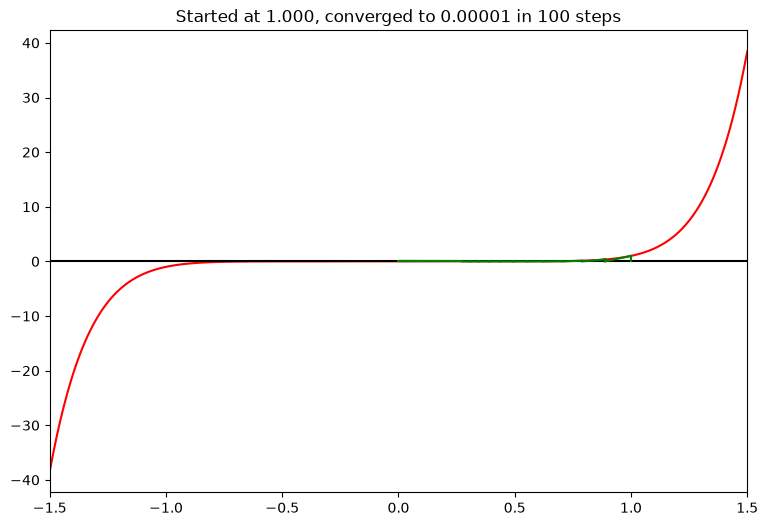
   0:  x =  0.88888888888889  err = 1.111111e-01
   5:  x =  0.49327018427257  err = 6.165877e-02
  10:  x =  0.27372990902883  err = 3.421624e-02
  15:  x =  0.15190065300101  err = 1.898758e-02
  20:  x =  0.08429407098405  err = 1.053676e-02
  25:  x =  0.04677722091831  err = 5.847153e-03
  30:  x =  0.02595803442990  err = 3.244754e-03
  35:  x =  0.01440486497991  err = 1.800608e-03
  40:  x =  0.00799367670345  err = 9.992096e-04
  45:  x =  0.00443592267809  err = 5.544903e-04
  50:  x =  0.00246162194645  err = 3.077027e-04
  55:  x =  0.00136602530002  err = 1.707532e-04
  60:  x =  0.00075804699540  err = 9.475587e-05
  65:  x =  0.00042066222875  err = 5.258278e-05
  70:  x =  0.00023343765198  err = 2.917971e-05
  75:  x =  0.00012954131281  err = 1.619266e-05
  80:  x =  0.00007188622564  err = 8.985778e-06
  85:  x =  0.00003989174824  err = 4.986469e-06
  90:  x =  0.00002213708626  err = 2.767136e-06
  95:  x =  0.00001228451019  err = 1.535564e-06
8.148481689595136e-06What this means for economics
Many of the pathological cases above rarely occur in practice
The ones that are real in economic applications are
multiple solutions
constraints on the domain of the function
the domain of attraction
It is therefore a good idea to combine a slow robust solver — to get into the domain of attraction — with the Newton method for fast convergence at the end
Successive approximations followed by Newton iterations is the classic approach in the estimation of dynamic programming models, namely the NFXP estimator of Rust (1987)
Multivariate Newton and optimization
Everything above is scalar, and everything above is about solving an equation.
But the natural multivariate problem in economics is not a system of equations — it is the first order condition of an optimization problem.
Consider with . The first order conditions for the interior optimum are
which is a system of equations in unknowns. Let’s use Newton-Raphson to solve it.
Derivation from the two-dimensional Taylor expansion
The scalar Newton step came from a first order Taylor expansion of around . In the optimization problems the step comes from a second order expansion of the objective — one order higher, because we are now looking for the gradient of the derivative in the FOC.
Take and write the step as . Around the current point ,
where every derivative is evaluated at . The right hand side is a quadratic in — a paraboloid — and we can find its stationary point exactly. Its two first order conditions are
which is a linear system for the step:
The matrix on the left is the Hessian , the vector on the right the gradient . Solving the system by hand,
and the iteration is the multivariate Newton method
Three observations before any code.
It is the scalar formula with replaced by . The scalar case is , nothing more.
The determinant sits in the denominator. It is the two-dimensional counterpart of in the scalar method: when the Hessian is close to singular the step explodes. Everything the failure-mode section said about applies to the determinant here.
The derivation used only the first order condition of the quadratic model. Nothing in it distinguishes a maximum from a minimum or a saddle point — a fact we will pay for below.
For a general system with the same argument on a first order expansion of gives
where is the Jacobian, the matrix of partial derivatives. Optimization is the special case , whose Jacobian is the Hessian .
An objective function with many critical points
Consider the following objective function which is the sum of four Gaussian bumps, one of which is a banana-shaped ridge:
with
def quad(x,y,c,d,A,B):
    '''Exponent q of a plain Gaussian bump, with its gradient and Hessian'''
    q   = (x-c)**2/A + (y-d)**2/B
    dq  = [2*(x-c)/A, 2*(y-d)/B]
    d2q = [[2/A+0*x, 0*x],[0*x, 2/B+0*x]]
    return q,dq,d2q

def quad_banana(x,y):
    '''Exponent q of the curved ridge, with its gradient and Hessian'''
    u = x - 0.55
    v = y - 0.63 + 2.5*u**2
    q   = u**2/0.055 + v**2/0.0025
    dq  = [2*u/0.055 + 4000*u*v, 800*v]
    d2q = [[2/0.055 + 4000*v + 20000*u**2, 4000*u],[4000*u, 800+0*x]]
    return q,dq,d2q

def bumps(x,y):
    '''The four terms of F: amplitude a, exponent q, and the derivatives of q'''
    return [(1.00,) + quad(x,y,0.22,0.27,0.018,0.030),
            (0.94,) + quad(x,y,0.73,0.25,0.080,0.012),
            (0.78,) + quad_banana(x,y),
            (1.20,) + quad(x,y,0.55,0.48,0.005,0.010)]

def F(x,y):
    return sum(a*np.exp(-q) for a,q,dq,d2q in bumps(x,y))
Source
plt.rcParams['figure.figsize'] = [9, 6]
def contour_plot(fun,levels=30,xlim=(0,1.2),ylim=(0,0.72),npoints=200,ax=None,clip=None):
    '''Contour plot of a function of two variables.
    With clip=p the levels are symmetric around zero and cut at the p-th percentile
    of |Z|, which keeps a few extreme values from swamping the picture.
    '''
    X,Y = np.meshgrid(np.linspace(*xlim,npoints),np.linspace(*ylim,npoints))
    Z = fun(X,Y)
    if clip is None:
        lv = np.linspace(Z.min(),Z.max(),levels)
        lv = np.concatenate([np.exp(np.linspace(np.log(Z.min()),np.log(0.2),levels//2)),np.linspace(0.3,Z.max(),levels//2)])
    else:
        c = np.percentile(np.abs(Z),clip)
        lv = np.linspace(-c,c,levels)
    if ax is None:
        fig, ax = plt.subplots()
    ax.contour(X,Y,Z,levels=lv)
    ax.set_aspect('equal','box')
    ax.set_xlim(*xlim)  # fix the window: paths drawn on top may leave it
    ax.set_ylim(*ylim)
    return ax

contour_plot(F)
plt.show()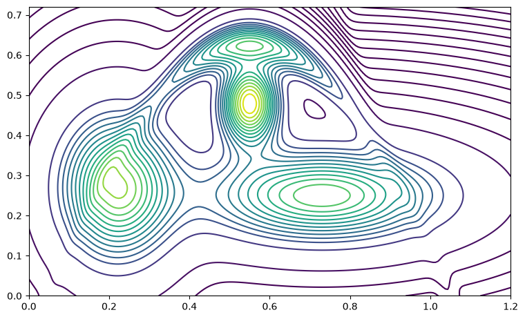
Three peaks, a ridge running over the top, and long flat plains towards the corners where all four exponentials have died out. A grid search over the square finds eleven critical points: four maxima, five saddle points and two minima.
The global maximum sits at , on the central peak.
Gradient and Hessian
Writing each term as saves us from differentiating four different functions. The chain rule gives, for each term,
so that
Only the derivatives of the exponents are left to compute. For a plain Gaussian term with ,
and for the ridge, writing and ,
The bumps() function above already returns , and for
all four terms, so the gradient and the Hessian of are two short loops:
def G(x,y):
    '''Gradient of F: grad(a exp(-q)) = -a exp(-q) grad(q)'''
    out = [0,0]
    for a,q,dq,d2q in bumps(x,y):
        g = a*np.exp(-q)
        for k in range(2):
            out[k] = out[k] - g*dq[k]
    return out

def H(x,y):
    '''Hessian of F: H(a exp(-q)) = a exp(-q) [grad(q) grad(q)' - H(q)]'''
    out = [[0,0],[0,0]]
    for a,q,dq,d2q in bumps(x,y):
        g = a*np.exp(-q)
        for k in range(2):
            for j in range(2):
                out[k][j] = out[k][j] + g*(dq[k]*dq[j] - d2q[k][j])
return outSource
eps = 1e-6
for x,y in [(0.30,0.70),(0.55,0.50),(0.80,0.20)]:
    Gn = [(F(x+eps,y)-F(x-eps,y))/(2*eps), (F(x,y+eps)-F(x,y-eps))/(2*eps)]
    Hn = [[(G(x+eps,y)[k]-G(x-eps,y)[k])/(2*eps) for k in range(2)],
          [(G(x,y+eps)[k]-G(x,y-eps)[k])/(2*eps) for k in range(2)]]
    print('at (%4.2f,%4.2f):  max |G-Gnum| = %.2e   max |H-Hnum| = %.2e'
          % (x,y,np.amax(np.abs(np.array(G(x,y))-np.array(Gn))),
                 np.amax(np.abs(np.array(H(x,y))-np.array(Hn).T))))
at (0.30,0.70): max |G-Gnum| = 5.77e-12 max |H-Hnum| = 1.25e-10
at (0.55,0.50): max |G-Gnum| = 5.39e-10 max |H-Hnum| = 7.92e-08
at (0.80,0.20): max |G-Gnum| = 4.54e-10 max |H-Hnum| = 1.65e-09
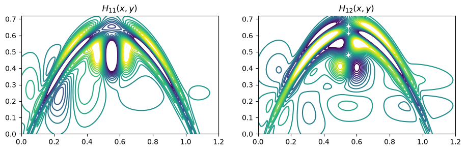
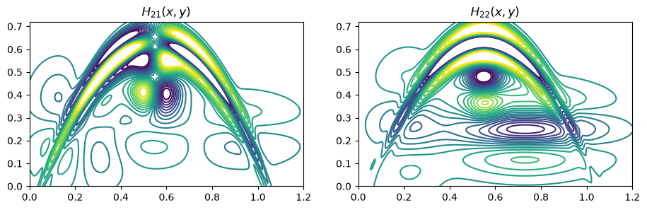
The two components of the gradient, and the four elements of the Hessian, are themselves functions of — the Newton step is a local linear approximation built from them at the current point. Note how much sharper their variation is than that of itself, and that and are the same picture, as they must be.
Source
fig, axs = plt.subplots(1,2,figsize=(11,5))
for k in range(2):
    contour_plot(lambda x,y: G(x,y)[k],ax=axs[k],clip=95,levels=20)
    axs[k].set_title('$G_%d(x,y)$'%(k+1))
plt.show()

fig, axs = plt.subplots(1,2,figsize=(11,10))
k=0
for j in range(2):
    contour_plot(lambda x,y: H(x,y)[k][j],ax=axs[j],clip=95,levels=20)
    axs[j].set_title('$H_{%d%d}(x,y)$'%(k+1,j+1))
plt.show()

fig, axs = plt.subplots(1,2,figsize=(11,10))
k=1
for j in range(2):
    contour_plot(lambda x,y: H(x,y)[k][j],ax=axs[j],clip=95,levels=20)
    axs[j].set_title('$H_{%d%d}(x,y)$'%(k+1,j+1))
plt.show()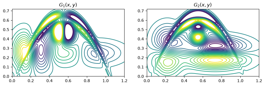
Multivariate Newton solver
The scalar solver carries over with two changes: the division becomes a linear solve, and the error is measured with a vector norm.
def newton2(fun,grad,x0,tol=1e-6,maxiter=100,callback=None):
    '''Newton method for solving a system of equations fun(x)=0,
    where x is a vector of 2 elements and grad is the Jacobian.
    Callback function is invoked at each iteration if given.
    '''
    # conversion to array function of array argument
    npfun  = lambda x: np.asarray(fun(x[0],x[1]))
    npgrad = lambda x: np.asarray(grad(x[0],x[1]))
    x0 = np.asarray(x0,dtype=float)
    for i in range(maxiter):
        x1 = x0 - np.linalg.solve(npgrad(x0),npfun(x0))  # matrix version
        err = np.amax(np.abs(x1-x0))  # vector sup norm
        if callback != None: callback(iter=i,err=err,x0=x0,x1=x1)
        if err<tol: break
        x0 = x1
    else:
        raise RuntimeError('Failed to converge in %d iterations'%maxiter)
    return x1
Source
def newton_path(x0,**kwargs):
    '''Solve G(x)=0 from x0, recording the sequence of Newton steps'''
    path = [np.asarray(x0,dtype=float)]
    xs = newton2(G,H,x0,callback=lambda **kw: path.append(kw['x1']),**kwargs)
    return xs, np.array(path)

def plot_newton_path(x0,**kwargs):
    '''Plot the Newton iterations on top of the contours of F'''
    xs, path = newton_path(x0,**kwargs)
    ax = contour_plot(F)
    ax.plot(path[:,0],path[:,1],c='r',marker='.')  # the path
    ax.scatter(*path[0],c='r',marker='o')          # starting point
    ax.scatter(*path[-1],c='b',marker='*',s=150,zorder=3)  # solution
    ax.set_title('Started at (%1.2f,%1.2f), converged in %d steps'%(*path[0],len(path)-1))
    plt.show()
Started just below the highest peak, the quadratic approximation is a good model of the objective and the solver walks straight up to it in four steps:
plot_newton_path([0.55,0.45])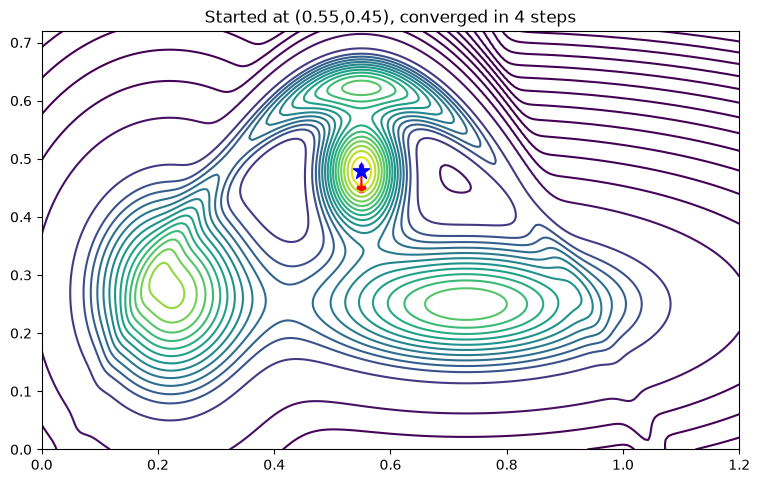
Now move the starting point down by 0.05, still on the flank of the same peak. The first step jumps 0.2 downward into the low ground between the two lower peaks, the second lands where is a fifteenth of its value at the start, and from there the method wanders back up and settles on a saddle point — not on the peak it started from:
plot_newton_path([0.55,0.40])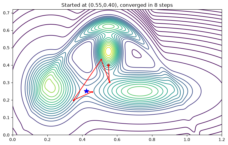
To see how little it takes, draw 10 Newton paths from random starting points in a small area
in the center. Stars mark the paths that converged and crosses the point where a run gave up —
for the plain solver most of those are far outside the picture, after maxiter=100 steps.
Source
def newton_trace(x0,solver=newton2,**kwargs):
    '''Newton path from x0, with the reason the solver stopped'''
    path = [np.asarray(x0,dtype=float)]
    try:
        solver(G,H,x0,callback=lambda **kw: path.append(kw['x1']),**kwargs)
        status = 'converged'
    except np.linalg.LinAlgError:
        status = 'singular Hessian'
    except RuntimeError as e:
        status = 'no ascent direction' if 'ascent' in str(e) else 'maxiter reached'
    return np.array(path), status

center, side = np.array([0.6,0.43]), 0.05  # the small square of starting points
starts = center + np.random.default_rng(44).uniform(-side/2,side/2,size=(10,2))
colors = plt.cm.autumn(np.linspace(0,0.85,len(starts)))  # slightly different colors

def plot_newton_paths(solver=newton2,starts=starts,colors=colors,**kwargs):
    '''Follow all the starting points at once, each path in its own color'''
    ax = contour_plot(F)
    for c,x0 in zip(colors,starts):
        path, status = newton_trace(x0,solver=solver,**kwargs)
        ax.plot(path[:,0],path[:,1],c=c,marker='.',lw=1.2,zorder=2)  # the path
        ax.scatter(*path[0],c=[c],marker='o',s=25,zorder=3)          # starting point
        if status == 'converged':
            ax.scatter(*path[-1],c=[c],marker='*',s=140,edgecolors='k',lw=.4,zorder=4)
        else:  # mark where the solver gave up
            ax.scatter(*path[-1],c=[c],marker='X',s=80,edgecolors='k',lw=.4,zorder=4)
    ax.scatter([],[],c='grey',marker='o',s=25,label='start')            # legend only
    ax.scatter([],[],c='grey',marker='*',s=140,edgecolors='k',lw=.4,label='converged')
    ax.scatter([],[],c='grey',marker='X',s=80,edgecolors='k',lw=.4,label='gave up')
    ax.legend(loc='upper left',fontsize=8,framealpha=0.8)
    plt.show()

plot_newton_paths()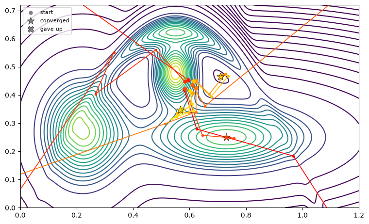
The starting points are withing a square of with side 0.05! Only a few paths converge, to different critical points; many leave the picture, several crossing directly over a peak on the way out without stopping at it.
Newton finds critical points, not maxima
The solver was given the first order condition , and that is all it knows. Any point satisfying it — a maximum, a minimum or a saddle point — is a solution, and which one is reached depends entirely on the starting value. The classification is ours to make afterwards, from the eigenvalues of the Hessian.
Source
for x0 in [(0.55,0.45),(0.55,0.40),(0.20,0.30),(0.75,0.25),
           (0.70,0.50),(0.55,0.65),(0.50,0.50),(0.10,0.80)]:
    try:
        xs, path = newton_path(x0)
        ev = np.linalg.eigvalsh(np.asarray(H(*xs)))  # Hessian at the solution
        kind = 'maximum' if (ev<0).all() else 'minimum' if (ev>0).all() else 'saddle'
        print('from (%4.2f,%4.2f) --> (%6.4f,%6.4f)  F = %5.3f  %-7s  in %2d steps'
              % (*x0,*xs,F(*xs),kind,len(path)-1))
    except RuntimeError as e:
        print('from (%4.2f,%4.2f) --> %s'%(*x0,e))
from (0.55,0.45) --> (0.5500,0.4787) F = 1.208 maximum in 4 steps
from (0.55,0.40) --> (0.4236,0.2526) F = 0.390 saddle in 8 steps
from (0.20,0.30) --> (0.2046,0.2902) F = 1.044 maximum in 5 steps
from (0.75,0.25) --> (0.7300,0.2500) F = 0.940 maximum in 3 steps
from (0.70,0.50) --> (0.7085,0.4660) F = 0.035 minimum in 5 steps
from (0.55,0.65) --> (0.5500,0.6227) F = 0.920 maximum in 6 steps
from (0.50,0.50) --> Failed to converge in 100 iterations
from (0.10,0.80) --> Failed to converge in 100 iterations
Two of the starting points above are 0.05 apart and end up at different critical points, one of them not even a maximum. What does that say about the domain of attraction of each solution?
How would you check, in code, that the point returned is the maximum you wanted?
What does a nearly singular Hessian do to the length of the step?
The lesson is the one from the scalar case, only sharper in higher dimensions: the failure modes do not go away, the domains of attraction are harder to picture, and the poly-algorithm remedy — a slow robust method first, Newton for the last digits — is correspondingly more valuable.
Line search and step size
Look again at the fan of paths above. What goes wrong is rarely the direction of the Newton step — near the current point the local quadratic approximation is a reasonable model, and it points the right way. What goes wrong is the length. The Newton step jumps all the way to the stationary point of the quadratic approximation, and when it is a poor description of further out, it lands somewhere unrelated to the problem.
The remedy is to keep the direction and shorten the step. Write the full Newton step as
and take
where is the step size. With this is the method we already have; with smaller it is a damped Newton step.
Choosing by step halving
The step size is chosen by trial: take the full step, check whether it improved matters, and if not, halve it.
Start with the full Newton step,
If the step improves on the current point, accept it and go on to the next iteration
If it does not, replace by
Repeat steps 2–3 until an improving step is found
The step sizes tried are therefore , so this is called a step-halving line search. It is computationally cheap: the gradient and the Hessian are computed once per iteration and reused for every trial — only the cheap part, the function value, is recomputed.
We are maximizing, so what counts as an improvement is the criterion function itself: a trial step is accepted when goes up. This turns the solver into a genuine maximizer — it can no longer converge to a minimum — but it only works if is an ascent direction, which requires the Hessian to be negative definite. Far from the optimum it need not be, and then no improves and the line search fails. Forcing the curvature matrix to be definite is exactly what the quasi-Newton methods listed at the end of these notes achieve.
def newton2_ascent(fun,grad,x0,obj=F,tol=1e-6,maxiter=100,maxhalve=25,callback=None):
    '''Newton method with a step-halving line search on the criterion obj.
    A step is accepted only when obj increases, so the iterations always climb.
    '''
    npfun  = lambda x: np.asarray(fun(x[0],x[1]))
    npgrad = lambda x: np.asarray(grad(x[0],x[1]))
    x0 = np.asarray(x0,dtype=float)
    obj0 = obj(*x0)  # criterion at the current point
    for i in range(maxiter):
        step = np.linalg.solve(npgrad(x0),npfun(x0))  # the full Newton step
        lam = 1.0
        for j in range(maxhalve):  # step-halving line search
            x1 = x0 - lam*step
            obj1 = obj(*x1)
            if obj1 > obj0: break  # uphill, accept this lambda
            lam = lam/2
        else:
            raise RuntimeError('No ascent direction at iteration %d'%i)
        err = np.amax(np.abs(x1-x0))
        if callback != None: callback(iter=i,err=err,x0=x0,x1=x1,lam=lam)
        if err<tol: break
        x0, obj0 = x1, obj1
    else:
        raise RuntimeError('Failed to converge in %d iterations'%maxiter)
    return x1
The same starting points, with a line search
Exactly the picture from above — the same ten starting points in the same small square, the same colors — but solved with the line search component.
Also a wider choice of starting points, line search can handle a few further out.
Source
plot_newton_paths(newton2_ascent)

center, side = np.array([0.5,0.4]), 0.5  # the small square of starting points
starts = center + np.random.default_rng(5).uniform(-side/2,side/2,size=(25,2))
colors = plt.cm.autumn(np.linspace(0,0.85,len(starts)))

plot_newton_paths(solver=newton2_ascent,starts=starts,colors=colors)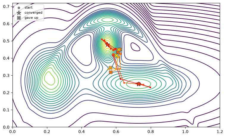
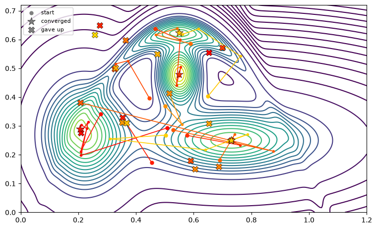
A completely different picture!
Nothing runs away: every path either climbs to a peak or stops, at a cross, where step halving could not find an uphill step.
The line search never returns a minimum or a saddle point — it cannot, because every accepted step increases and neither is approached from below.
The line search is also the only one of the two that reaches the global maximum from this cluster of starting points, and it does so in fewer iterations, having halved the step on just three of them.
The price is multiple failures. They are not failures to converge: the solver stops because no improved , which happens whenever the Newton direction is not an ascent direction.
That is a property of the direction, not of the step length, and shortening the step cannot cure it. The points uphill only when the Hessian is negative definite, which far from a peak it need not be.
Plain Newton converges more often, but half of what it returns is not a maximum. Is a method that more often gives up (fails to find suitable step size) better or worse?
Would step halving have rescued any of the failures of the one-dimensional Newton?
The full step is tried first at every iteration, and is only halved when Newton is going off. What implications does this have for the convergence properties of the method?
BFGS, BHHH and other quasi-Newton methods
The line search of the previous section can only work if the direction it is handed points uphill, and does so only where the Hessian is negative definite. Quasi-Newton methods remove that condition by never using the true Hessian at all: they carry an approximation to it, built from the gradients already computed, and update that approximation in a way that preserves its definiteness at every iteration. The direction is then an improving one by construction, and the line search always has a step to find.
BFGS (Broyden–Fletcher–Goldfarb–Shanno) builds up an approximation to the inverse Hessian iteratively, ensuring correct definiteness (negative for maximization and positive for minimization problems). Other approaches to approximating the Hessian, such as the DFP (Davidon–Fletcher–Powell) method, were developed for general optimization problems.
BHHH (Berndt-Hall-Hall-Hausman) gets the same guarantee out of statistics rather than out of the update formula.
Maximizing a log-likelihood with score contributions , it uses the outer product in place of . That matrix is positive semi-definite by construction, and by the information identity it estimates , so the step
always climbs. BHHH, being based on the statistical properties of the scores, is more specific to econometric M-estimation problems — and for that reason it is often not found in standard optimization packages.
Regions of attraction of the four-hills function
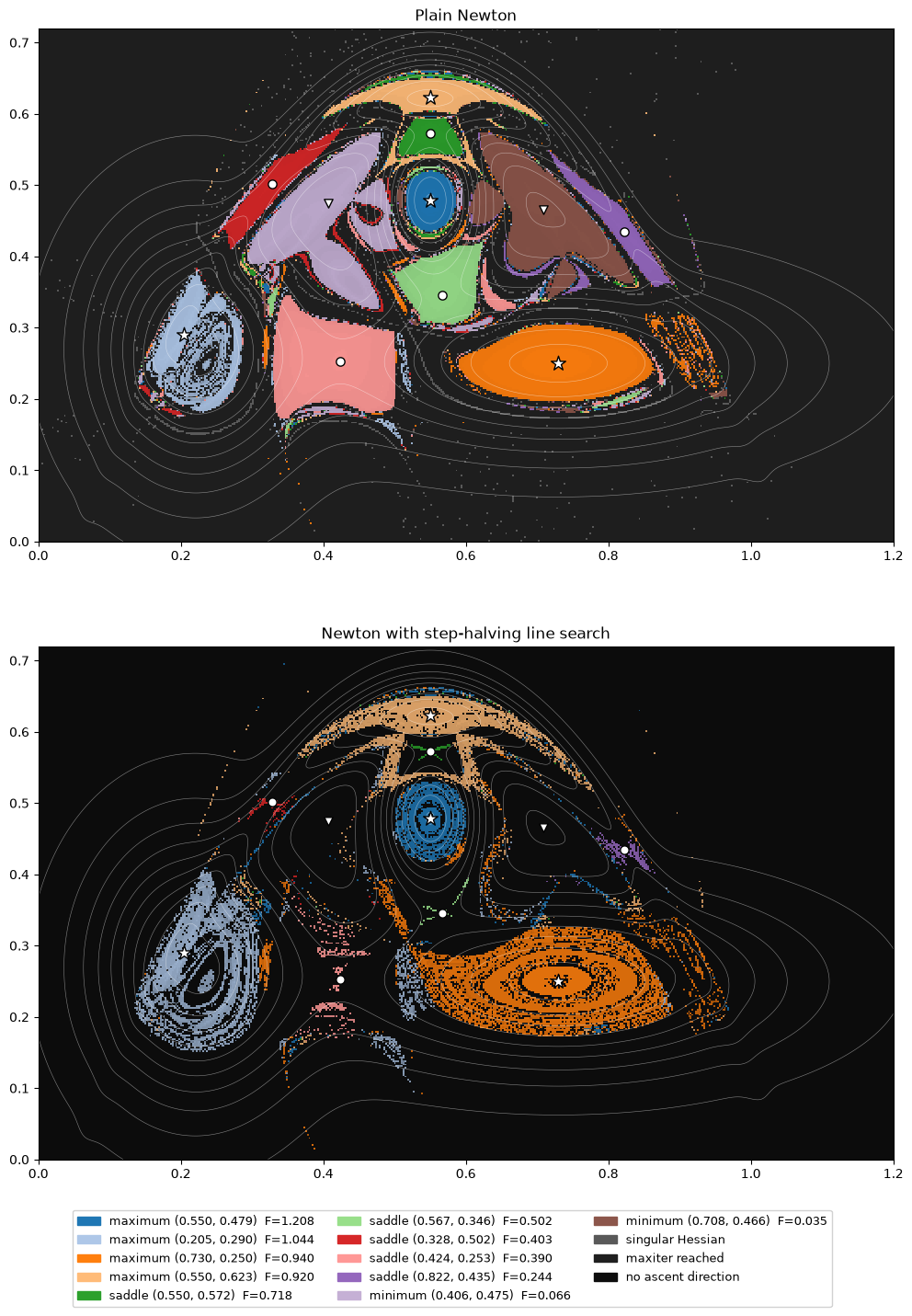
The solution of homework delta_newton_fractals: every starting point of a grid covering the picture is
iterated at once, in the same vectorized style as the cubic example in the task notebook.
Source
from matplotlib.patches import Patch

def newton_grid(X,Y,ascent=False,tol=1e-6,maxiter=100,maxhalve=25):
    '''Newton's method for grad F = 0 from every point of the grid (X,Y) at once.
    With ascent=True the full step is halved until F increases, so the runs always climb.
    Returns endpoints x, y, the iteration count, and a status code for every run:
    0 converged, 1 singular Hessian, 2 maxiter reached, 3 no ascent direction.
    '''
    x, y   = X.astype(float).copy(), Y.astype(float).copy()  # current position of every run
    iters  = np.zeros(X.shape,dtype=int)
    status = np.full(X.shape,2)                   # 'maxiter reached' unless stopped earlier
    active = np.ones(X.shape,dtype=bool)          # runs still going
    f0 = F(x,y) if ascent else None               # criterion at the current point
    with np.errstate(all='ignore'):               # inf/nan on runaway points are caught below
        for i in range(maxiter):
            g0, g1 = G(x,y)                       # gradient: two arrays over the grid
            (a, b), (c, d) = H(x,y)               # Hessian: four arrays over the grid
            s = np.maximum.reduce([np.abs(a),np.abs(b),np.abs(c),np.abs(d)])  # scale of H
            a, b, c, d, g0, g1 = a/s, b/s, c/s, d/s, g0/s, g1/s  # normalize, see the note above
            det = a*d - b*c
            dx = (d*g0 - b*g1)/det                # the 2x2 solve H^{-1} g written out
            dy = (a*g1 - c*g0)/det
            bad = active & ~(np.isfinite(dx) & np.isfinite(dy))  # det=0 or overflow
            status[bad], iters[bad] = 1, i+1
            active &= ~bad
            if ascent:                            # step-halving line search, all runs at once
                lam = np.ones(X.shape)
                for j in range(maxhalve):
                    x1, y1 = x - lam*dx, y - lam*dy
                    f1 = F(x1,y1)
                    uphill = f1 > f0
                    if (uphill | ~active).all(): break   # every live run climbs
                    lam[~uphill] /= 2             # halve only where it does not yet
                else:
                    noasc = active & ~uphill
                    status[noasc], iters[noasc] = 3, i+1
                    active &= ~noasc
                dx, dy = lam*dx, lam*dy           # the step actually taken
            else:
                x1, y1 = x - dx, y - dy
            err = np.maximum(np.abs(dx),np.abs(dy))   # sup norm of the step
            done = active & (err < tol)
            status[done], iters[done] = 0, i+1
            x[active], y[active] = x1[active], y1[active]  # move only the live runs
            if ascent: f0 = np.where(active,f1,f0)
            active &= ~done
            if not active.any(): break
    return x, y, iters, status

def critical_points(x,y,tol=1e-3):
    '''Distinct points among the endpoints x,y, sorted maxima first then by F,
    together with their type from the eigenvalues of the Hessian'''
    pts = np.unique(np.round(np.column_stack([x,y]),6),axis=0)  # collapse identical endpoints
    crit = []
    for p in pts:                                # merge the ones within tol of each other:
                                                 # the 1e-6 step test leaves endpoints ~1e-4 apart around a saddle
        if not crit or np.abs(np.array(crit)-p).max(axis=1).min() > tol:
            crit.append(p)
    crit = np.array(crit)
    ev = np.array([np.linalg.eigvalsh(np.asarray(H(*p))) for p in crit])
    kind = np.where((ev<0).all(axis=1),'maximum',np.where((ev>0).all(axis=1),'minimum','saddle'))
    rank = {'maximum':0,'saddle':1,'minimum':2}
    order = np.lexsort((-F(*crit.T),[rank[k] for k in kind]))
    return crit[order], kind[order]

FAIL = ['singular Hessian','maxiter reached','no ascent direction']  # status codes 1,2,3

def classify(x,y,status,crit):
    '''Index of the critical point each run reached, or len(crit)+status-1 if it failed'''
    dist = np.abs(np.stack([x,y],axis=-1)[...,None,:]-crit).max(axis=-1)  # (ny,nx,ncrit)
    which = dist.argmin(axis=-1)
    return np.where(status==0, which, len(crit)+status-1)

xlim, ylim = (0,1.2), (0,0.72)   # the window of the contour plots in the chapter

def grid(nx):
    '''Grid of starting points covering the window with square pixels'''
    ny = round(nx*(ylim[1]-ylim[0])/(xlim[1]-xlim[0]))
    return np.meshgrid(np.linspace(*xlim,nx),np.linspace(*ylim,ny))

def basins_plot(X,Y,x,y,iters,status,crit,kind,ax,title):
    '''Color the grid of starting points by the critical point each run reached'''
    which = classify(x,y,status,crit)
    ncrit = len(crit)
    colors = np.vstack([plt.cm.tab20(np.arange(ncrit) % 20)[:,:3],  # critical points
                        [[.35,.35,.35],[.12,.12,.12],[.05,.05,.05]]])  # the three failure modes
    rgb = colors[which]                                    # (ny,nx,3) image
    conv = status==0
    shade = np.ones(X.shape)
    shade[conv] = 0.5 + 0.5*(1-iters[conv]/iters[conv].max())  # lighter = fewer iterations
    ax.imshow(rgb*shade[...,None],extent=[*xlim,*ylim],origin='lower',interpolation='nearest')
    ax.contour(X,Y,F(X,Y),levels=np.linspace(0.05,1.2,12),colors='white',linewidths=0.4,alpha=0.5)
    for marker,k in [('*','maximum'),('o','saddle'),('v','minimum')]:
        m = kind==k
        ax.scatter(crit[m,0],crit[m,1],c='white',edgecolors='black',marker=marker,
                   s=140 if k=='maximum' else 45,zorder=3)
    ax.set_xlim(*xlim); ax.set_ylim(*ylim)
    ax.set_title(title)
    labels = ['%s (%.3f, %.3f)  F=%.3f'%(k,*p,F(*p)) for p,k in zip(crit,kind)] + FAIL
    present = np.unique(which)
    return [Patch(color=colors[i],label=labels[i]) for i in present]

X, Y = grid(500)
%time xn, yn, itn, stn = newton_grid(X,Y)               # plain Newton
%time xa, ya, ita, sta = newton_grid(X,Y,ascent=True)   # with the line search

crit, kind = critical_points(np.r_[xn[stn==0],xa[sta==0]],np.r_[yn[stn==0],ya[sta==0]])
print('%d critical points found\n'%len(crit))
print('%-8s %8s %8s %7s %14s %14s'%('type','x','y','F','plain Newton','line search'))
wn, wa = classify(xn,yn,stn,crit), classify(xa,ya,sta,crit)
for i,(p,k) in enumerate(zip(crit,kind)):
    print('%-8s %8.4f %8.4f %7.4f %13.1f%% %13.1f%%'%(k,*p,F(*p),100*(wn==i).mean(),100*(wa==i).mean()))
for j,f in enumerate(FAIL):
    print('%-32s %13.1f%% %13.1f%%'%(f,100*(stn==j+1).mean(),100*(sta==j+1).mean()))

fig, axes = plt.subplots(2,1,figsize=(12,16))
handles  = basins_plot(X,Y,xn,yn,itn,stn,crit,kind,axes[0],'Plain Newton')
handles += basins_plot(X,Y,xa,ya,ita,sta,crit,kind,axes[1],'Newton with step-halving line search')
seen = {}                                          # one legend entry per category
for h in handles: seen.setdefault(h.get_label(),h)
fig.legend(seen.values(),seen.keys(),loc='upper center',bbox_to_anchor=(0.5,0.08),ncol=3,fontsize=9,framealpha=0.9)
plt.show()
CPU times: user 5.81 s, sys: 248 ms, total: 6.06 s
Wall time: 6.07 s
CPU times: user 4.81 s, sys: 118 ms, total: 4.93 s
Wall time: 5.02 s
11 critical points found

type            x        y       F   plain Newton    line search
maximum    0.5500   0.4787  1.2085           0.7%           1.1%
maximum    0.2046   0.2902  1.0443           1.7%           2.5%
maximum    0.7300   0.2500  0.9400           3.0%           4.0%
maximum    0.5500   0.6227  0.9202           1.2%           2.0%
saddle     0.5500   0.5722  0.7181           0.6%           0.1%
saddle     0.5667   0.3456  0.5019           1.3%           0.0%
saddle     0.3285   0.5019  0.4032           1.0%           0.1%
saddle     0.4236   0.2526  0.3898           2.9%           0.2%
saddle     0.8223   0.4350  0.2440           0.8%           0.1%
minimum    0.4064   0.4749  0.0663           3.1%           0.0%
minimum    0.7085   0.4660  0.0351           2.8%           0.0%
singular Hessian                           1.2%           0.0%
maxiter reached                           79.7%           0.0%
no ascent direction                        0.0%          89.9%
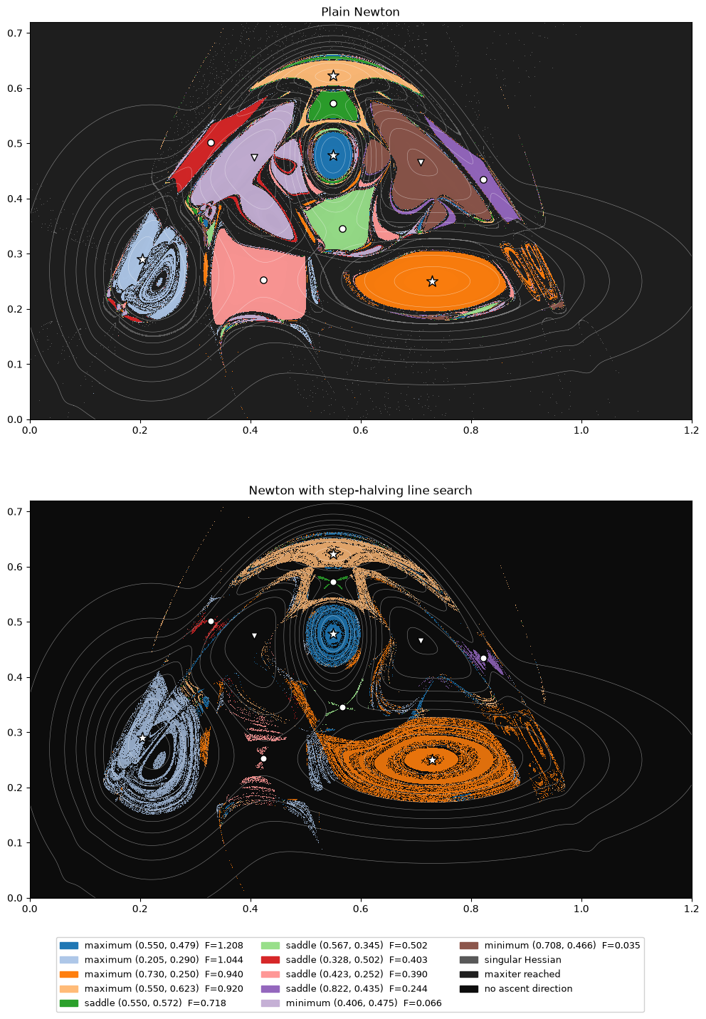
Same regions at higher resolution (5000 points on x-axis)
- Rust, J. (1987). Optimal Replacement of GMC Bus Engines: An Empirical Model of Harold Zurcher. Econometrica, 55(5), 999. 10.2307/1911259
- Judd, K. L. (1998). Numerical Methods in Economics (p. 633). MIT Press. https://mitpress.mit.edu/9780262100717/numerical-methods-in-economics/
- Adda, J., & Cooper, R. W. (2023). Dynamic Economics: Quantitative Methods and Applications. MIT Press. https://mitpress.mit.edu/9780262547888/dynamic-economics
- Berndt, E. R., Hall, B. H., Hall, R. E., & Hausman, J. A. (1974). Estimation and Inference in Nonlinear Structural Models. In Annals of Economic and Social Measurement, Volume 3, Number 4 (Vol. 3, pp. 653–665). National Bureau of Economic Research. https://www.nber.org/chapters/c10206