📖 Cake eating on and off a grid and function approximation

So far every dynamic choice in the course was discrete, and the maximum in the Bellman equation was taken over a short list. With a continuous choice the maximum is an optimization problem in every state! We will learn a few solution techniques for the models with continuous choice in the next few classes before addressing the estimation of these models. Along the way we need to remind ourselves of function approximation.

cd sb-dse-code
git reset --hard HEAD
git pull

git pull upstream main                         # collect the task
cp -r tasks/iota_deaton solutions/iota_deaton  # work on the copy

Cake eating¶

The cake eating problem has the structure of the all so important consumption-savings model and an analytic solution, so every numerical method can be checked against the truth.

• Choice: how much cake $c_t$ to eat in period $t = 0, 1, \dots, \infty$

• State: the size of the cake $W_t$, with $W_0$ given

• Transition: what is not eaten is left for the future, $W_{t+1} = W_t - c_t$

• Preferences: flow utility $u(c_t) = \log(c_t)$ and discount factor $\beta \in (0,1)$

The consumer maximizes the discounted utility over the whole horizon,

Look how easy it is to get the familiar Bellman equation in this case. Let

The last equation is due to the fact that infinitely many time periods look the same from the point of view of today and tomorrow. Realizing further that in this case nothing can depend on index of time, we can drop the time index to arrive at

The right-hand side defines the Bellman operator $T(V)(W)$ from space of value functions to itself

• operator $T$ is a contraction by Blackwell’s sufficient conditions, as in Class 8

• therefore the value function iterations (VFI) $V_{i} = T(V_{i-1})$ converge to the unique solution from any starting point

The question of this class is how to compute $T(V)$ when $c$ and $W$ are continuous.

The analytic solution¶

Let $u(c) = \log(c)$, what is the solution?

The consumer eats a constant fraction $1-\beta$ of what is left, every period.

The analytic solution exists only because the model is so simple

• only few models admit an analytical solution

• more complicated models require backward induction by hand + spotting the regularities before actual guessing

Its value, at least here, as well as any analytic property is the ability to verify numerical methods

Solving on a grid¶

The simplest numerical approach replaces both the state and the choice with a finite grid, $\vec{W} = \{W_1, \dots, W_n\}$ on $[0, \overline{W}]$. To avoid evaluating $V$ between grid points, make the next period cake the decision variable so we have:

• here $i$ denotes the iteration of the VFI algorithm

Every term is known on the grid, so one iteration is a maximum over an $n \times n$ matrix of choices, exactly as in the discrete models of the earlier classes:

import numpy as np
import matplotlib.pyplot as plt

class cake_ongrid():
    '''Cake eating on a grid: the next period cake is chosen from the state grid'''

    def __init__(self, beta=.9, Wbar=10, ngrid=50):
        self.beta = beta                               # discount factor
        self.Wbar = Wbar                               # upper bound on cake size
        self.ngrid = ngrid                             # number of grid points
        self.epsilon = np.finfo(float).eps             # smallest positive float
        self.grid = np.linspace(self.epsilon, Wbar, ngrid)   # grid for both state and choice

    def bellman(self, V0):
        '''Bellman operator, V0 is a vector of values on the grid'''
        c = self.grid - self.grid[:, np.newaxis]       # states in columns, next cake in rows
        c[c == 0] = self.epsilon                       # avoid log(0) when nothing is eaten
        mask = c > 0                                   # feasible choices: eat a positive amount
        matV1 = np.full((self.ngrid, self.ngrid), -np.inf)   # -inf marks infeasible choices
        matV0 = np.repeat(V0.reshape(self.ngrid, 1), self.ngrid, 1)   # V0 of the next cake, in rows
        matV1[mask] = np.log(c[mask]) + self.beta * matV0[mask]       # maximand of the Bellman equation
        V1 = np.amax(matV1, axis=0)                    # maximum in every column
        c1 = self.grid - self.grid[np.argmax(matV1, axis=0)]          # optimal consumption
        return V1, c1

    def solve(self, maxiter=1000, tol=1e-4, callback=None):
        '''Value function iterations'''
        V0 = np.log(self.grid)                         # start from eating everything
        for i in range(maxiter):
            V1, c1 = self.bellman(V0)
            if callback: callback(iter=i, grid=self.grid, value=V1, policy=c1)
            if np.all(abs(V1 - V0) < tol):
                break
            V0 = V1
        else:
            raise RuntimeError('No convergence: maximum number of iterations achieved')
        return V1, c1

Source

def check_analytic(model, title=''):
    '''Plot the numerical solution of a cake eating model against the analytic one'''
    b = model.beta
    aV = lambda w: np.log(w)/(1-b) + np.log(1-b)/(1-b) + b*np.log(b)/(1-b)**2
    aP = lambda w: (1-b)*w
    xg = np.linspace(model.Wbar/1000, model.Wbar, 1000)   # dense grid for the analytic solution
    V, policy = model.solve()
    fig, (ax1, ax2) = plt.subplots(1, 2, figsize=(12, 4.5))
    ax1.plot(model.grid[1:], V[1:], label='numerical')
    ax1.plot(xg, aV(xg), label='analytic')
    ax2.plot(model.grid, policy, label='numerical')
    ax2.plot(xg, aP(xg), label='analytic')
    for ax, t in ((ax1, 'Value function'), (ax2, 'Policy function')):
        ax.set(xlabel='Cake size, W', title=t)
        ax.grid(color='0.9')
        ax.legend()
    fig.suptitle(title)
    plt.show()
    return np.max(np.abs(policy - aP(model.grid)))

err = check_analytic(cake_ongrid(beta=0.9, Wbar=10, ngrid=100), 'Same grid for state and choice, 100 points')
print(f'Largest error in consumption: {err:.3f}')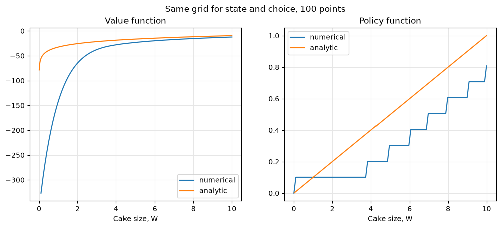

Largest error in consumption: 0.293

The value function is close, but the policy is a staircase. On this grid the consumer can only eat the difference of two grid points, so with 100 points on $[0,10]$ every consumption level is a multiple of about 0.1, whatever the true optimum.

Where it breaks: the choice set is tied to the state grid. Refining the state grid is the only way to refine the choices, the cost of one iteration grows with $n^2$, and in a model where next period’s state is not a grid point at all, the trick is not available. That is the case as soon as savings earn interest or income is random.

Function approximation¶

Any method that separates the choice from the state grid needs the value function between grid points. The interpolation problem: given nodes $a = x_0 < x_1 < \dots < x_n = b$ and the values $f(x_i)$ of an unknown function, find a function $s$ from a chosen class with $s(x_i) = f(x_i)$ for all $i$, and use $s(x)$ in place of $f(x)$ at any $x \in [a,b]$.

• Interpolation matches the data exactly: the approximation passes through every $(x_i, f(x_i))$. This is what a solver needs, because the data are computed exactly.

• Curve fitting finds the central tendency of noisy data, as in regression, with more data points than parameters. Better fitted for the situations with (potential) measurement errors.

• Extrapolation, evaluating the approximation/fitted curve outside the initial domain $[a, b]$, should be avoided unless the theoretical properties of $f$ are known there. A wider grid is almost always the better fix.

The quality of an approximation is measured in the uniform norm aka infinity norm, $\lVert f - s \rVert_\infty = \max_{x \in [a,b]} |f(x) - s(x)|$, the largest error anywhere on the interval, which is what matters when $s$ stands in for $f$ inside a solver.

There are two families of methods:

• connect the dots piece by piece, or

• replace $f$ by one simpler function on the whole interval (which could still connect all dots to interpolate)

Splines¶

• linear splines: order 2, degree 1, continuous

• quadratic splines: order 3, degree 2, continuous first derivative

• cubic splines: order 4, degree 3, continuous first and second derivatives

To compute spline interpolation one would need to solve the following system:

• passing through both ends on $n$ intervals = $2n$ equations

• continuous derivatives on $n-1$ interior knots = $(n-1)(k-2)$ equations

• number of coefficients for one interval = $k$

• total number of unknowns = $nk$

• $2n+(n-1)(k-2)=nk-k+2$ equations

• $k-2$ additional boundary conditions on the derivatives at $a$ and $b$

Linear interpolation is the spline of order 2: continuous, with kinks at the knots.

• on $[x_i, x_{i+1}]$ it is $s(x) = f(x_i) + \frac{f(x_{i+1}) - f(x_i)}{x_{i+1} - x_i}(x - x_i)$, and

• for a twice continuously differentiable $f$ and the largest spacing $h = \max_i (x_{i+1} - x_i)$,

Halving the spacing divides the error by four.

The cubic spline, need two boundary conditions

• $s''(a) = s''(b) = 0$ for the natural spline, or

• the slopes $s'(a) = f'(a)$, $s'(b) = f'(b)$ for the clamped spline.

The coefficients solve a tridiagonal linear system, at a cost proportional to $n$.

For a clamped spline and $f$ with four continuous derivatives,

so halving the spacing divides the error by sixteen.

In Python both are available:

• np.interp for the linear spline

• scipy.interpolate.CubicSpline for the cubic spline

Polynomial approximation¶

A polynomial of degree $n$ through $n+1$ distinct nodes exists and is unique.

How good it is (in terms of approximation error) depends on where the nodes are.

The error has two factors.

• first depends only on $f$.

• second, the node polynomial $\prod_i (x - x_i)$, depends only on the nodes, and it is the one we control.

1. With equally spaced nodes the node polynomial is small in the middle of the interval and grows rapidly towards its ends.

For functions whose derivatives grow fast, such as $f(x) = 1/(1+25x^2)$ on $[-1,1]$, the error near the ends grows without bound as $n$ increases: the Runge phenomenon. More nodes make the approximation worse.

2. The nodes that make $\max_{x \in [-1,1]} \big|\prod_i (x - x_i)\big|$ smallest are the zeros of the Chebyshev polynomial $T_{n+1}$, where the maximum equals $2^{-n}$, its smallest possible value.

The error bound becomes $\lVert f - p_n \rVert_\infty \leqslant \dfrac{\lVert f^{(n+1)} \rVert_\infty}{2^n (n+1)!}$.

The Chebyshev polynomials are

or equivalently

The $n+1$ zeros of $T_{n+1}$, Chebyshev nodes, are

They cluster towards the ends of $[-1,1]$.

The polynomials are orthogonal with respect to the weight $(1-z^2)^{-1/2}$, and also discretely orthogonal on the Chebyshev nodes, so the interpolating polynomial $p_n(z) = \sum_{k=0}^{n} c_k T_k(z)$ has explicit coefficients, no linear system needed:

A general interval $[a,b]$ is mapped to $[-1,1]$ by $z = 2(x-a)/(b-a) - 1$, as in the flexible logit of Class 13.

For $f$ with $k$ continuous derivatives, Chebyshev interpolation of degree $n$ satisfies Judd, 1998

which falls faster than any power of $n$ when $f$ is smooth: Chebyshev interpolation is within a logarithmic factor of the best polynomial approximation in the uniform norm.

The four methods side by side, first with 12 nodes on a function with some curvature, then with a growing number of nodes on the Runge function:

Source

from scipy import interpolate
from numpy.polynomial import polynomial, chebyshev
import warnings

def approximations(f, a, b, n):
    '''Linear spline, cubic spline, polynomial on equal nodes and Chebyshev interpolation with n nodes'''
    xe = np.linspace(a, b, n)                          # equally spaced nodes
    with warnings.catch_warnings():
        warnings.simplefilter('ignore')                # polyfit warns about poor conditioning
        p = polynomial.polyfit(xe, f(xe), n-1)
    return {'linear spline':           lambda x: np.interp(x, xe, f(xe)),
            'cubic spline':            interpolate.CubicSpline(xe, f(xe)),
            'polynomial, equal nodes': lambda x: polynomial.polyval(x, p),
            'Chebyshev, own nodes':               chebyshev.Chebyshev.interpolate(f, n-1, domain=[a, b])}

f = lambda x: np.exp(-x/4)*np.sin(x) + 1/(1 + x**2)   # function to approximate
a, b, n = -5, 10, 12                                   # interval and number of nodes
xd = np.linspace(a, b, 1000)                           # dense grid to measure errors
fig, (ax1, ax2) = plt.subplots(2, 1, figsize=(14, 16))
ax1.plot(xd, f(xd), 'k', lw=2, label='f(x)')
ax1.scatter(np.linspace(a, b, n), f(np.linspace(a, b, n)), c='k', zorder=3)
for name, g in approximations(f, a, b, n).items():
    ax1.plot(xd, g(xd), label=name)
    ax2.semilogy(xd, np.abs(g(xd) - f(xd)) + 1e-16, label=name)
ax1.set(ylim=(-1.5, 2), title=f'{n} nodes')
ax2.set(ylim=(1e-6, 15), title='Absolute error')
for ax in (ax1, ax2):
    ax.legend(fontsize=8); ax.grid(color='0.9')
plt.show()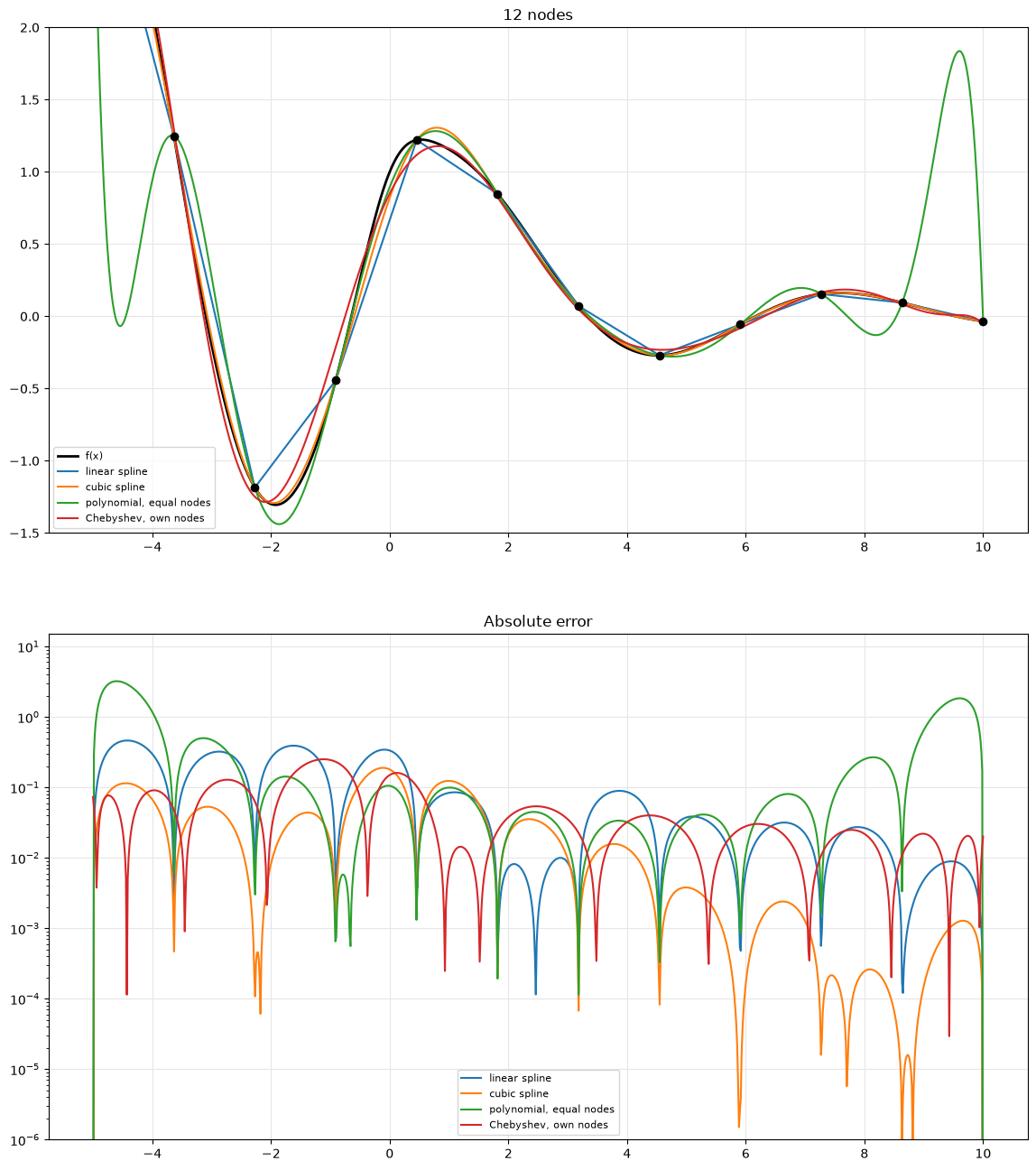

In economic models we control the three things that determine the accuracy:

• the number of nodes, more is better, at a cost in every iteration of the solver

• the location of the nodes, denser where the function curves more: the error bounds scale with the derivatives of $f$, which for the log-utility value function are largest near zero wealth

• the type of the approximation, matched to the function: smooth functions favor Chebyshev polynomials, functions with kinks favor splines, because the bounds above need the derivatives to exist

Where it breaks:

• polynomials and cubic splines do not preserve monotonicity or concavity, so an approximated value function can have a local maximum that the true one does not

• linear interpolation preserves both, which is why it is the default in the solvers below, despite its lower accuracy.

• in several dimensions all of these methods generalize as tensor products, but the number of nodes grows exponentially with the dimension. Curse of dimentionality

• taking derivatives of the approximations usually make little sense, much better to compute and interpolate the derivative function ⚠️

Discretized choice with interpolation¶

With an interpolated value function the choice no longer has to live on the state grid.

Keep the grid $\vec{W}$ for the state, and give the choice its own grid $\vec{D}(W_j)$ for every state point.

Scale to the feasible interval $[0, W_j]$ so that the constraint $0 \leqslant c \leqslant W$ is respected by construction:

where $\hat V_{i-1}$ is the interpolated value function and $i$ denotes the VFI iteration index

class cake_discretized():
    '''Cake eating with a separate choice grid and interpolated value function'''

    def __init__(self, beta=.9, Wbar=10, ngrid=50, nchgrid=100):
        self.beta = beta                               # discount factor
        self.Wbar = Wbar                               # upper bound on cake size
        self.ngrid = ngrid                             # number of points on the state grid
        self.nchgrid = nchgrid                         # number of points on the choice grid
        self.epsilon = np.finfo(float).eps             # smallest positive float
        self.grid = np.linspace(self.epsilon, Wbar, ngrid)   # grid for the state
        self.share = np.linspace(self.epsilon, 1, nchgrid)   # choices as shares of the cake

    def bellman(self, V0):
        '''Bellman operator, V0 is a vector of values on the state grid'''
        c = self.share[:, np.newaxis] * self.grid      # choices in rows, scaled to [0,W] in each column
        W1 = self.grid - c                             # next period cake, off the grid in general
        matV1 = np.log(c) + self.beta * np.interp(W1, self.grid, V0)   # linear interpolation of V0
        i = np.argmax(matV1, axis=0)                   # optimal choice in every column
        return matV1[i, np.arange(self.ngrid)], c[i, np.arange(self.ngrid)]

    solve = cake_ongrid.solve                          # the same value function iterations

Source

err = check_analytic(cake_discretized(beta=0.9, Wbar=10, ngrid=100, nchgrid=100),
                     'Separate choice grid, 100 + 100 points')
print(f'Largest error in consumption: {err:.3f}')
print(f'{"state grid":>10} {"choice grid":>12} {"max error in c":>15}')
for ng, nch in ((50, 50), (100, 100), (100, 500), (500, 100), (500, 500)):
    m = cake_discretized(beta=0.9, Wbar=10, ngrid=ng, nchgrid=nch)
    V, c = m.solve()
    print(f'{ng:>10} {nch:>12} {np.max(np.abs(c - (1-m.beta)*m.grid)):>15.4f}')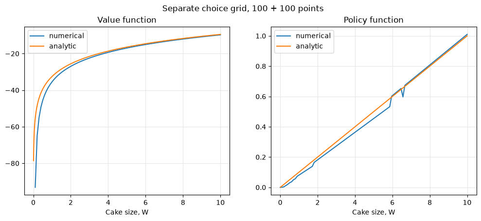

Largest error in consumption: 0.060
state grid  choice grid  max error in c
        50           50          0.1162
       100          100          0.0597

       100          500          0.0365
       500          100          0.0106

       500          500          0.0121

The policy is now five times closer to the truth with the same number of points. The table shows that both grids matter. A choice grid of $n_c$ shares pins consumption down to within $W/n_c$, but here the grid of shares happens to contain a point within 0.001 of the optimal share $1-\beta$, so most of the remaining error comes from the interpolation of $\hat V$ on the state grid. The error is not even monotone in the grid sizes, a warning against reading accuracy off a single run.

How to increase the accuracy further:

• more points on both grids, at a cost of $n \times n_c$ evaluations per iteration

• choice grids that respect the constraints of the model, as above

• state grid points relocated to where the value function curves most

• a better approximation of $\hat V$, or no discretization of the choice at all: the next class maximizes over a continuous $c$ in every state, and solves the first order condition instead

The consumption-savings model¶

The cake eating model becomes the workhorse consumption-savings model of Deaton (1991) once savings earn interest and the consumer has an income:

• $M$ is wealth at the beginning of the period, cash on hand

• $0 \leqslant c \leqslant M$: consumption cannot exceed wealth, the consumer cannot borrow

• $R$ is the gross return on savings and $\tilde{y}$ next period’s income, both of which can be random

• $u(c) = \log(c)$ and the discount factor $\beta$ as before

Cake eating is the special case $R = 1$ and $\tilde{y} = 0$.

The timing of the model separates the choice from the uncertainty:

Savings $A$, the post-decision state, carry all the information about the current period that next period needs, and the constraint $0 \leqslant c \leqslant M$ is the same as $0 \leqslant A \leqslant M$.

Computing expectations¶

Let income be log-normal, $\log\tilde{y} \sim N(0, \sigma^2)$, so $\tilde{y} > 0$ and $\mathbb{E}\tilde{y} = \exp(\sigma^2/2)$. The expectation in the Bellman equation is an integral, and it has to be computed at every state and every choice on every iteration. We approximate it by quadrature, a weighted sum over fixed nodes $y_k$ with weights $\omega_k$:

How to choose the nodes and the weights, and how quadrature compares with Monte Carlo integration, is covered in Class 16.

Both discretized solvers carry over to this model, with one difference. On the grid, next period wealth is chosen from the state grid and consumption is backed out as $c = M - (M' - y)/R$, which works only when income is deterministic: with random income $M'$ is not a choice, so the on-grid trick fails. With a choice grid, consumption is the choice and $\hat V$ is interpolated at $M' = R(M-c) + y_k$ for every quadrature node.

The Euler equation¶

The first order condition for an interior choice and the envelope theorem,

give $V'(M) = u'(c^\star(M))$, and together the Euler equation

The marginal utility of consuming today equals the discounted expected marginal utility of saving it and consuming tomorrow. When the borrowing constraint binds, $c^\star = M$ and the left side is larger. The Euler equation holds for the exact solution, whichever method computed it, so it is the basis of the solvers of the next two classes and of the accuracy checks for all of them.

Checking the accuracy of a solution¶

The cake eating model has an analytic solution; the consumption-savings model does not. Two checks still measure the accuracy of any numerical solution: a special case of the model with a sharp prediction, and the Euler equation, which holds at every point.

Constant consumption: Keane’s test¶

Take the deterministic model, $\tilde{y} = y$ with certainty, and let $\beta R = 1$. Then the Euler equation becomes

so as long as the borrowing constraint does not bind, consumption is the same in every period. Along such a path wealth must also stay constant, otherwise it diverges. From $M_0 \geqslant y$ the consumer eats the annuity value of the wealth,

and saves $A = (M_0 - y)/R \geqslant 0$, so the constraint never binds.

Keane’s test uses this prediction: solve the deterministic model with $\beta R = 1$ numerically, simulate the consumer from some initial wealth, and check that the simulated consumption profile is flat, at the level $c^\star$. An accurate solver passes. An inaccurate one produces consumption that drifts up or down over time. The error of the policy function accumulates through wealth, so the test magnifies small errors that a plot of the policy function hides.

The test is cheap and has a known answer, but it checks the solution only along the simulated paths, and only for one parameter combination. It is a necessary condition for an accurate solver, not a sufficient one.

Euler equation residuals¶

The Euler equation holds for the exact solution at every point where the borrowing constraint does not bind, at any parameter values. For a numerical policy $c(M)$, interpolated between the grid points, the relative Euler equation residual

measures how far the policy is from satisfying it, as a fraction of marginal utility. It is computed on a grid much denser than the solver’s, to catch the errors between the grid points, and only where $c(M) < M$: at a corner solution the Euler equation holds as an inequality, and the residual is not an error.

The two checks complement each other. The Euler residuals apply at any parameter values and at every point of the state space, but only to one step of the dynamics. The constant consumption check applies to one special case, but follows the errors as they accumulate over a whole simulated path. The homework runs both on the two solvers with discretized choice of this class.