📖 Conditional choice probabilities, identification and two-step estimator
Class 12 — Thursday, October 1
NFXP solves the model inside every likelihood evaluation. This class turns the argument around: the conditional choice probabilities (CCPs) observed in the data pin down the value function differences, so the model can be estimated without ever solving it. The same result of Hotz & Miller (1993) also says exactly what the data can and cannot identify.
Running the code for this lecture
Every code example below is also a runnable notebook in the course code repository,
in the folder session12-oct1/.
You should have cloned that repository already — if not, the instructions are in the algorithms and complexity lecture.
Update your copy before the class. Editing a file in place makes git pull refuse to
update it, so discard whatever you changed while experimenting:
cd sb-dse-code
git reset --hard HEAD
git pull
Nothing in this repository is submitted, so experiment freely — but copy anything you want to keep out of it first, or commit that to a branch of your own.
Setting up the Python environment is covered in Python.
Homework eta_ccp: recovering value differences from choice data
Graded homework: task eta_ccp in the class repository. Collect it and work on a
copy in your own repository:
git pull upstream main                 # collect the task
cp -r tasks/eta_ccp solutions/eta_ccp  # work on the copy
Derive the Bellman equation of the Zurcher model in the space of integrated value
functions and implement it as a subclass zurcher_ccp of the model class, checking that
it is a contraction. Then verify numerically, at the NFXP estimates and a handful of
other parameter values, the Hotz–Miller inversion and the Arcidiacono–Miller
relationship between the integrated value function, the choice-specific values and the
choice probabilities.
The notebook ccp_representations.ipynb in the task folder loads the model class, the
NFXP estimator and Zurcher’s data from session10-11/ of the code repository, and has
the details of the task, step by step. The code of Class 10, session10-11/ in the code
repository, is worth having beside you while you work.
Submit it as a pull request, following the git workflow. One of you presents a solution at the start of the next Tuesday class.
Integrated expected value function
Maintain the setup of the Zurcher engine replacement model of Rust (1987) from Class 9, leaning to more generality. The Bellman equation of the Zurcher problem is
and it breaks into three pieces that are useful on their own: the choice-specific value, the expected value, and the value function itself,
The last equation uses the EV1 assumption on the distribution of , but in more generality it can be written as
Let’s repeat the terminology:
is the choice-specific value function, or conditional value function, and
is commonly referred to as the expected value function and sometimes as the ex-post value function
Here is a new object and yet another representation. The integrated value function , also known as the ex-ante value function, is the value function with the taste shock integrated out,
The subscript follows the notation of Aguirregabiria & Mira (2007), who define it as the value function under a strategy profile .
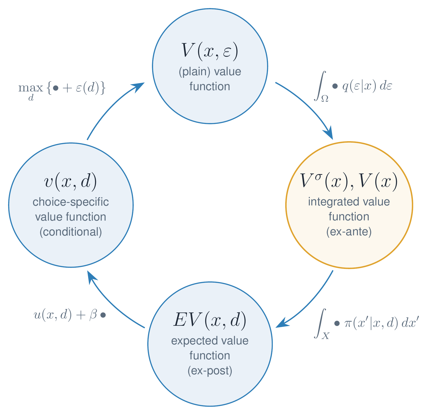
The Bellman circle of value functions: plain value function , integrated value function , expected value function and choice-specific value function
We could write the Bellman equation in the space of integrated value functions by cutting the circle of Bellman at a different point:
The new representation of the Bellman equation is
This is the expectation of the maximum utility in a RUM with alternative utilities given by , which McFadden (1974) called the social surplus function in Class 6.
In the EV1 case max-stability gives it in closed form, with the Euler–Mascheroni constant,
Choice probabilities
Recall that by the Williams–Daly–Zachary theorem in the general case the choice probabilities are the derivatives of the social surplus function,
and under the EV1 assumption the derivative of the logsum is the multinomial logit,
Exchanging the order of differentiation and integration in the general case, we can also express the choice probabilities as the integral with respect to the distribution of the indicator that is the maximizer
Inversion theorem
Let denote the reference alternative, so that the values of other alternatives will be measured relative to it.
For each consider the vector of value differences , where is the number of alternatives, with elements
Rewriting the event from above step by step, we have
The steps are:
write the argmax as a system of inequalities,
subtract from both sides of each inequality so that only differences appear, and
read the result as the probability mass of a region of that depends on only
Compare this derivation to the static multinomial logit model of Class 6.
In other words, if
is a mapping from value differences to the vector of probabilities, then the choice probabilities are given by .
The theorem is the reason the reference alternative was needed: probabilities that sum to one carry degrees of freedom, and so do the differences. Levels of the choice-specific values are not recoverable from choices, only their differences.
What we have: the Hotz–Miller inversion gives a mapping from the choice probabilities to the value differences for any choice model with random terms satisfying the regularity conditions of the theorem, and in the EV1 and GEV cases we have closed-form expressions for the inverse map.
Why is a reference alternative needed, and does the choice of matter?
What happens to the inverse map when an estimated is exactly zero at some , and how likely is that with frequency estimates on the bus data?
Relationship between , and choice probabilities
Recall that the choice probability in the general case is simply the expectation of the indicator that a particular choice yields the maximum utility,
The expression for as the expected maximum can then be expanded using the law of iterated expectations, conditioning on which alternative is chosen:
Conditional on being the maximizer, the maximum is , and is not random, which is all that happens between the second and the last line. The term that remains,
has the special name of correction term, see Aguirregabiria & Mira (2002). It is the expectation of the random component conditional on the event that the alternative it is associated with has the highest value. We end up with
We can make one more step, using the Hotz–Miller inversion with a reference alternative , to arrive at
where is a function of the choice probabilities and not of the value functions, see Lemma 1 in Arcidiacono & Miller (2011). This result holds can be written for any reference alternative , and therefore holds for every .
In other words, the difference between the integrated value function and any choice-specific reference value is a function of the choice probabilities only. This is the result that every CCP-based method builds on.
Correction terms for EV1 and GEV
Hotz & Miller (1993) and Arcidiacono & Miller (2011) show that the correction term has a closed form in the two workhorse cases,
where is the set of alternatives in the same nest as and is the scale parameter within the nest.
Finite dependence
Hotz-Miller inversion establishes the relationship between the choice probabilities and the value differences, but values are still defined recursively.
Main idea of finite dependence is to note that it may be possible to cancel out the future after several periods
recursion reduces to several periods (one repeated cycle)
then no fixed point to solve for
estimator can be applied to short panels
The idea goes back to Altuğ & Miller (1998), and we follow the general version in Section 3 of Arcidiacono & Miller (2011).
The starting point is the expression derived above
Substituting it into the definition of the choice-specific value gives
where is just some alternative chosen in the next period.
It does not have to be the same in every .
It does not even have to be a single alternative either, and can be represented by some choice weights , such that :
Let’s now repeat this step again in the next period, and so on. This is referred to as telescoping the integrated value function.
Fix the current period , the state and the initial choice .
A choice sequence assigns to every later period and every state a vector of decision weights with .
The weights may depend on the state reached and may mix over alternatives
Arcidiacono & Miller (2011) write them as
Along the sequence, the state evolves according to the distribution
of , defined recursively by
In other words, we look at the distribution of states resulting from the chosen sequence of choice weights
or in the simple case of a deterministic sequence of choices
In both cases the induced distribution of states is
Now we can compute the choice specific value along some choice sequence!
Theorem 1 of Arcidiacono & Miller (2011) shows that, for any state , any initial choice and any choice sequence,
The term compensates at each step for the sequence not being the optimal policy.
Why is this useful?
From period on, set the weights of the two sequences equal.
Every term of Theorem 1 after is then identical for and and cancels in the difference, leaving
Helpful properties of finite dependence:
the mappings, the first-stage CCPs and the transition probabilities, the value difference is a linear function of flow utilities over periods.
only the functions of alternatives that carry positive weight in one of the two sequences are needed
The Zurcher model is the leading case: engine replacement is a renewal action, so the model has one-period finite dependence. The practical of Class 13 derives the resulting value difference and codes the estimator built on it.
Finite dependence can take more than one period and require sequences that react to the state. In the stylized labor-supply example of Section 3.2.2 of Arcidiacono & Miller (2011), working today raises human capital by 1 or 2 units with equal probability. Working in any later period raises it by exactly 1, and staying home leaves it unchanged. Starting with home, the sequence work, work reaches at for sure. Starting with work, stay home at if the gain was 2 and work if it was 1, then stay home at : again at . The pair has two-period finite dependence, and the second sequence is state-contingent.
What if no finite dependence?
Finite dependence is a property of the transition probabilities, and nothing guarantees it. If no later choice can undo or replicate the effect of today’s choice on the state, the terms never cancel. Then the infinite sum, or the matrix inversion of the identification section, is back.
Finding the sequences by hand is application-specific; Arcidiacono & Miller (2019) search for the decision weights numerically.
See also the JMP by Jaepil Lee (2025) for an application of numerically searching for finite dependence sequences in estimation.
The CCPs that enter are those at the states reachable within periods, including rarely visited ones, where is noisy. The pay-off is largest in nonstationary models with short panels. There, the CCPs in the last observed period carry all the information about the unobserved future, and flow utilities are estimable up to periods before the sample ends without modeling the horizon.
For bus engines does replacement constitute a renewal action, and what does depend on?
Which CCPs does the Zurcher model require, and at which mileages are they expected to be poorly estimated in the bus data?
Think of a model in your own field. Does it have a renewal or terminal action, and if not, what would a finite-dependence sequence look like?
Identification
The previous results have immediate implications for identification of the model primitives of dynamic discrete choice models in general.
The model is characterized by the primitives (and the horizon, infinite here)
The data are a panel of states and choices
The question is: which primitives the data pin down??
Assumption: the discount factor and the distribution of the taste shocks are taken as known
Further, consistent estimate of the transition probabilities are available (see below).
So, main focus is non-parametric identification of flow utilities !
Assume a discrete state space, so that the integral over is a sum and can be represented by a matrix multiplication. As before, the transition probability matrix for the state space under action .
First, we can consistently estimate the choice probabilities , the CCPs, and the transition probabilities from the data on in the first stage, giving common name CCP or two-stage estimators to the whole family of CCP-based estimation methods.
Now fix the reference alternative and let its flow utility be given for every . Stack all entities into vectors over the state space .
The definition of the choice-specific value and the relationship give
This is the integrated value function in terms of first-stage objects and the flow utility of the reference alternative .
To recover the utility of the other actions, follow the same route from and :
and substituting ,
The same result can be written without matrix inversion, as a discounted sum along a choice sequence, using Theorem 1 above:
take the sequence that chooses in every period after , for
let be the distributions of the state it generates after the initial choice
How does this relate to what we already have?
It is the matrix formula above written out term by term
It is Theorem 1 of the finite dependence section applied to and with the same continuation, and differenced
From the matrix formula to the sum
Split and expand . The row of is , which gives exactly the sum in the theorem.
Why is this useful?
When the two sequences reach the same distribution of the state after periods, the sum stops at .
is then identified from CCPs at most periods ahead
this is what makes identification off short panels possible in nonstationary models
The converse matters as much. Arcidiacono & Miller (2020) also show that any bounded choice of , state by state, together with the implied by the formula above, generates exactly the same CCPs and transitions as the true model: the two are observationally equivalent.
In the matrix form, replacing by an arbitrary vector changes the other utilities to
without changing anything in the data. Therefore:
flow utilities are identified only relative to one alternative per state
the normalization does not have to set it to zero, nor use the same alternative in every state
a normalization is needed unless some data inform the level of utility, for example data on costs or prices
or unless the parameterization of restricts how utilities vary across states and alternatives tightly enough to rule out the transformation above
A parametric form alone is not enough: if it is flexible enough to absorb , the normalization is still implicit in it.
In the Zurcher model, and . Which normalization does this correspond to?
The derivation takes as given. Where exactly does it enter, and why can it not be recovered from the same equations?
Which counterfactuals survive a change of the normalization, and which do not?
CCP-based estimation
There are many estimation approaches based on the CCP representation of the dynamic discrete choice models:
Minimum distance Altuğ & Miller, 1998
Simulated moments Hotz et al., 1994
Asymptotic least squares Pesendorfer & Schmidt-Dengler, 2008
Quasi-maximum likelihood Hotz & Miller, 1993
Pseudo-maximum likelihood Aguirregabiria & Mira, 2002
Nested pseudo-likelihood Aguirregabiria & Mira, 2007
Many-many more
All of them share the same two-step structure, which is why they are collectively called two-step CCP estimators:
Input: panel data (x_it, d_it)
Algorithm:
  1. Estimate the CCPs P(d|x) and transition probabilities Π(d) directly from the data
     - non-parametrically, like frequency counts
     - parametrically, like multinomial logit or nested logit for P(d|x)
       and a discrete choice model for Π(d)
     - semi-parametrically, like flexible or local logit
  2. Use the estimated CCPs and transition probabilities to construct
     a criterion function that depends on the structural parameters θ
  3. Optimize the criterion function to obtain the estimates of θ
     by one of the approaches above
Output: estimate of θ, obtained without solving the model
The second step is where the methods differ: the value function differences implied by and the first-stage estimates are matched to the first-stage CCPs by a distance, a set of moments, or a likelihood. In the Zurcher model with the logit inverse map, step 1 estimates the replacement probability in every mileage bin, a frequency table in principle and a smoothed one in practice, and step 2 is a static logit estimation with the future differenced out by finite dependence. This is what we code in the practical of Class 13, and the pseudo-likelihood versions of step 2 are the subject of Class 14.
Issues with CCP-based estimation
The first-stage estimates enter the criterion function directly, so their sampling error is inherited by .
With many states and a modest panel, frequency estimates of are noisy or exactly zero in rarely visited states, and in the inverse map amplifies the noise.
Two-step estimators are therefore less efficient than NFXP in finite samples, and in the tails of the state space they can be badly biased.
Smoothing the first stage helps, at the price of a choice of smoother that the theory does not make for you.
What are the strengths of CCP-based estimation, and how does it compare to NFXP?
What are the potential weaknesses and difficulties of this approach?
Further topics
The CCP estimation approach gave rise to a number of further avenues of methodological research and applied work:
Unobserved heterogeneity among decision-makers, Arcidiacono & Miller (2011), who developed the theory of representation with correction terms and an expectation-maximization algorithm to estimate finite mixtures of types
Computational finite dependence: find and exploit the finite dependence structure in applications by comparing the distributions of future states at different points of the state space, Arcidiacono & Miller (2019)
Identification literature: the discount factor by Abbring & Daljord (2020), and further special cases and circumstances
- Hotz, V. J., & Miller, R. A. (1993). Conditional Choice Probabilities and the Estimation of Dynamic Models. The Review of Economic Studies, 60(3), 497–529. 10.2307/2298122
- Arcidiacono, P., & Miller, R. A. (2011). Conditional Choice Probability Estimation of Dynamic Discrete Choice Models With Unobserved Heterogeneity. Econometrica, 79(6), 1823–1867. 10.3982/ECTA7743
- Rust, J. (1987). Optimal Replacement of GMC Bus Engines: An Empirical Model of Harold Zurcher. Econometrica, 55(5), 999. 10.2307/1911259
- Aguirregabiria, V., & Mira, P. (2007). Sequential Estimation of Dynamic Discrete Games. Econometrica, 75(1), 1–53. 10.1111/j.1468-0262.2007.00731.x
- McFadden, D. (1974). Conditional logit analysis of qualitative choice behavior. Frontiers in Econometrics.
- Aguirregabiria, V., & Mira, P. (2002). Swapping the Nested Fixed Point Algorithm: A Class of Estimators for Discrete Markov Decision Models. Econometrica, 70(4), 1519–1543. 10.1111/1468-0262.00340
- Altuğ, S., & Miller, R. A. (1998). The effect of work experience on female wages and labour supply. The Review of Economic Studies, 65(1), 45–85. https://academic.oup.com/restud/article-abstract/65/1/45/1589921
- Arcidiacono, P., & Miller, R. A. (2019). Nonstationary dynamic models with finite dependence. Quantitative Economics, 10(3), 853–890. 10.3982/QE626
- Lee, J. (2025). A Structural Analysis of Opioid Misuse: Health, Labor, Policy, and Misperception of the Risk of Opioid Misuse. https://raw.githubusercontent.com/jaepillee0315/jaepillee0315.github.io/master/_drafts/Jaepil_Lee_JMP.pdf
- Arcidiacono, P., & Miller, R. A. (2020). Identifying dynamic discrete choice models off short panels. Journal of Econometrics, 215(2), 473–485. 10.1016/j.jeconom.2018.12.025
- Kalouptsidi, M., Scott, P. T., & Souza-Rodrigues, E. (2021). Identification of counterfactuals in dynamic discrete choice models. Quantitative Economics, 12(2), 351–403. 10.3982/QE1253
- Abbring, J. H., & Daljord, Ø. (2020). Identifying the discount factor in dynamic discrete choice models. Quantitative Economics, 11(2), 471–501. 10.3982/QE1352
- Hotz, V. J., Miller, R. A., Sanders, S., & Smith, J. (1994). A simulation estimator for dynamic models of discrete choice. The Review of Economic Studies, 61(2), 265–289.
- Pesendorfer, M., & Schmidt-Dengler, P. (2008). Asymptotic Least Squares Estimators for Dynamic Games -super-1. The Review of Economic Studies, 75(3), 901–928. https://econpapers.repec.org/scripts/a/abstract.pf?h=RePEc:oup:restud:v:75:y:2008:i:3:p:901-928;terms=Least%20Squares%20Estimators%20of%20Dynamic%20Games
- Aguirregabiria, V., & Mira, P. (2010). Dynamic discrete choice structural models: A survey. Journal of Econometrics, 156(1), 38–67. 10.1016/j.jeconom.2009.09.007