🔬 Practice: one model, three solvers

Today we code the stochastic consumption-savings model of Class 15, compare ways to compute the expectation over income, and solve the model three ways: value function iterations with a discretized choice, value function iterations with a continuous choice, and time iterations on the Euler equation. Then we measure what each solver buys, in accuracy and in time, with two checks that apply to any solution method.

Running the code for this lecture

The code for this class is in the folder session16-oct20/ of the course code repository. We write it together in class, starting from the pre-code notebook deaton_pre.ipynb, which has the model object and the headings but not the solvers. The complete notebook deaton.ipynb has all the code of this page.

You should have cloned that repository already — if not, the instructions are in the algorithms and complexity lecture.

Update your copy before the class. Editing a file in place makes git pull refuse to update it, so discard whatever you changed while experimenting:

cd sb-dse-code
git reset --hard HEAD
git pull

Nothing in this repository is submitted, so experiment freely — but copy anything you want to keep out of it first, or commit that to a branch of your own.

Setting up the Python environment is covered in Python.

The model object¶

The model of Deaton (1991), from Class 15:

V(M) = \max_{0 \leqslant c \leqslant M} \Big\{ \log(c) + \beta\, \mathbb{E}_{y}\, V\big(R(M - c) + \tilde{y}\big) \Big\}, \qquad \log\tilde{y} \sim N(0, \sigma^2)

The model object holds the parameters, the state grid on $(0, \overline{M}]$ , the choice grid as shares of wealth, the quadrature nodes and weights for the income, and the primitives: utility and the budget constraint. Every solver below is a function of this object.

import time
import numpy as np
import matplotlib.pyplot as plt
from scipy.stats import lognorm
from scipy.optimize import minimize_scalar, brentq

class deaton():
    '''Stochastic consumption-savings model of Deaton (1991) with log-normal income'''

    def __init__(self, beta=0.9, R=1.05, sigma=0.5, Mbar=10, ngrid=100, nchgrid=250, nquad=10):
        self.beta, self.R, self.sigma = beta, R, sigma   # discount factor, gross return, income std
        self.Mbar = Mbar                                  # upper bound of the state grid
        self.ngrid, self.nchgrid, self.nquad = ngrid, nchgrid, nquad
        self.eps = np.finfo(float).eps                    # smallest positive float
        self.grid = np.linspace(self.eps, Mbar, ngrid)    # state grid on (0, Mbar]
        self.share = np.linspace(self.eps, 1, nchgrid)    # choice grid as shares of wealth
        x, w = np.polynomial.legendre.leggauss(nquad)     # Gauss-Legendre nodes and weights on [-1,1]
        self.quadp = lognorm.ppf((x + 1) / 2, sigma)      # income nodes y_k = F^{-1}(q_k)
        self.quadw = w / 2                                # weights, sum to one

    def u(self, c):
        return np.log(c)                                  # utility

    def next_wealth(self, M, c, y):
        return self.R * (M - c) + y                       # budget constraint

def interp(x, xp, fp):
    '''Linear interpolation, extrapolated linearly beyond the last grid point'''
    slope = (fp[-1] - fp[-2]) / (xp[-1] - xp[-2])
    return np.where(x > xp[-1], fp[-1] + slope * (x - xp[-1]), np.interp(x, xp, fp))

The last row of the grid is a linear extrapolation: with random income, next period wealth can exceed $\overline{M}$ , and np.interp would silently hold the function constant there.

Computing expectations¶

Income is log-normal, $\log\tilde{y} \sim N(0, \sigma^2)$ , so $\tilde{y} > 0$ and $\mathbb{E}\tilde{y} = \exp(\sigma^2/2)$ . The expectation in the Bellman equation is an integral, and it has to be computed at every state and every choice on every iteration, so the method matters. There are two families: quadrature, a weighted sum over fixed nodes, and Monte Carlo integration, an average over random draws.

\mathbb{E}_y V(RA + \tilde y) = \int V(RA + y)\, dF(y) \approx \sum_{k=1}^{K} \omega_k\, V(RA + y_k)

Newton–Cotes rules approximate the integrand on equally spaced nodes by a polynomial, and integrate the polynomial. With nodes spaced $h$ apart on $[a,b]$ , the composite trapezoid rule, linear pieces between neighboring nodes, and Simpson’s rule, quadratic pieces over pairs of intervals, have errors

-\frac{(b-a)\,h^2}{12} f''(\xi) \qquad\text{and}\qquad -\frac{(b-a)\,h^4}{180} f^{(4)}(\xi)

for some $\xi \in [a,b]$ : the same rates as linear and cubic splines, and for the same reason.

Gaussian quadrature chooses the nodes as well as the weights, which doubles the degree of polynomials it integrates exactly. The nodes come from orthogonal polynomials.

Definition

Let $w(x) > 0$ be a weight function on an interval $[a,b]$ , possibly unbounded, with finite moments $\int_a^b x^k w(x)\, dx$ for all $k$ . It defines the inner product

\langle f, g \rangle_w = \int_a^b f(x)\, g(x)\, w(x)\, dx

A family of polynomials $\{\phi_k\}_{k=0}^{\infty}$ , with $\phi_k$ of degree exactly $k$ , is orthogonal with respect to $w$ if

\langle \phi_i, \phi_j \rangle_w = 0 \;\text{ for } i \neq j, \qquad \langle \phi_k, \phi_k \rangle_w > 0,

and orthonormal if in addition $\langle \phi_k, \phi_k \rangle_w = 1$ .

the Chebyshev polynomials of Class 15 are the orthogonal family for $w(x) = (1-x^2)^{-1/2}$ on $[-1,1]$

Theorem (Gaussian quadrature)

Let $\{\phi_k\}$ be the polynomials orthogonal with respect to a weight function $w(x) > 0$ on $[a,b]$ , with $\phi_k$ of degree $k$ and leading coefficient $q_k$ .

Let the nodes $x_1 < \dots < x_n$ be the $n$ zeros of $\phi_n$ , which all lie in $(a,b)$ , and the weights $\omega_i = -\dfrac{q_{n+1}/q_n}{\phi_n'(x_i)\,\phi_{n+1}(x_i)} > 0$ .

Then for $f$ with $2n$ continuous derivatives, for some $\xi \in [a,b]$ ,

\int_a^b f(x)\, w(x)\, dx = \sum_{i=1}^{n} \omega_i f(x_i) + \frac{f^{(2n)}(\xi)}{q_n^2\, (2n)!}

In particular the rule is exact for all polynomials of degree up to $2n - 1$ .

Each weight function gives a family of rules, with nodes and weights tabulated in numpy.polynomial:

Gauss–Legendre: $w(x) = 1$ on $[-1,1]$ , for integrals over a bounded interval
Gauss–Chebyshev: $w(x) = (1-x^2)^{-1/2}$ on $[-1,1]$ , nodes $x_i = \cos\big(\tfrac{2i-1}{2n}\pi\big)$ and equal weights $\pi/n$
Gauss–Hermite: $w(x) = e^{-x^2}$ on $(-\infty, \infty)$ , for expectations with respect to the normal distribution
Gauss–Laguerre: $w(x) = e^{-x}$ on $[0, \infty)$ , for exponential discounting

For our log-normal income, Gauss–Hermite fits exactly. With $\tilde y = e^{\sigma Z}$ , $Z \sim N(0,1)$ , and the change of variable $z = \sqrt{2}\,x$ ,

\mathbb{E}\, g(\tilde y) = \frac{1}{\sqrt{\pi}} \int_{-\infty}^{\infty} g\big(e^{\sqrt{2}\sigma x}\big)\, e^{-x^2} dx \approx \sum_{i=1}^{n} \frac{\omega_i}{\sqrt{\pi}}\, g\big(e^{\sqrt{2}\sigma x_i}\big)

with $(x_i, \omega_i)$ the Gauss–Hermite nodes and weights.

A second rule works for any distribution with an invertible CDF: change the variable to $q = F(y)$ , which is uniform on $[0,1]$ , and apply Gauss–Legendre there, with nodes $y_k = F^{-1}(q_k)$ and the weights rescaled to $[0,1]$ . It is convenient, but the integrand in $q$ , $g\big(F^{-1}(q)\big)$ , has unbounded derivatives at $q = 0$ and $q = 1$ , so the error term of the theorem gives no fast convergence. The model object above uses this rule.

Monte Carlo integration replaces the integral by an average over $N$ independent draws $y_i$ from $F$ :

\mathbb{E}\, g(\tilde y) \approx \frac{1}{N} \sum_{i=1}^{N} g(y_i)

By the law of large numbers the average converges to the expectation, and by the central limit theorem its error is approximately normal with standard deviation $\sigma_g/\sqrt{N}$ , $\sigma_g^2 = \operatorname{Var} g(\tilde y)$ , estimated by the sample standard deviation divided by $\sqrt N$ . The rate $1/\sqrt{N}$ is slow, four times as many draws for twice the precision, but it does not depend on the dimension of the integral, while the number of nodes of a product quadrature rule grows exponentially with it.

Example: an expectation with a known value

Let $\tilde y$ be log-normal, $\log \tilde y \sim N(0, \sigma^2)$ , with $\sigma = 0.5$ .

Then $1/\tilde y$ is log-normal too, $\log(1/\tilde y) = -\log \tilde y \sim N(0, \sigma^2)$ , so

\mathbb{E}\,(1/\tilde y) = \exp(\sigma^2/2)

exactly, and the error of any numerical method can be measured.

The code computes $\mathbb{E}\,(1/\tilde y)$ three ways and reports the absolute errors:

Gauss–Hermite, with nodes $y_i = e^{\sqrt{2}\sigma x_i}$ and weights $\omega_i/\sqrt{\pi}$ from the formula above, for $n = 3, 5, 10, 20$ nodes
Gauss–Legendre on the CDF, with nodes $y_k = F^{-1}(q_k)$ and weights rescaled to $[0,1]$ , for the same numbers of nodes
Monte Carlo, with $N$ = 100 to 100 000 draws, next to its estimated standard error

def quadrature_hermite(sigma, n):
    '''Gauss-Hermite nodes and weights for expectations of functions of a log-normal income'''
    x, w = np.polynomial.hermite.hermgauss(n)          # weight exp(-x^2) on the real line
    return np.exp(np.sqrt(2) * sigma * x), w / np.sqrt(np.pi)   # nodes y_k, weights sum to one

def quadrature_cdf(sigma, n):
    '''Gauss-Legendre on the CDF: nodes y_k = F^{-1}(q_k)'''
    x, w = np.polynomial.legendre.leggauss(n)          # Gauss-Legendre on [-1,1]
    return lognorm.ppf((x + 1) / 2, sigma), w / 2      # rescaled to [0,1], weights sum to one

sigma = 0.5
exact = np.exp(sigma**2 / 2)                           # E(y) = E(1/y) = exp(sigma^2/2)
print(f'{"nodes":>7} {"Gauss-Hermite":>14} {"Legendre on CDF":>16}   errors in E(1/y)')
for n in (3, 5, 10, 20):
    errs = [abs(w @ (1 / y) - exact) for y, w in (quadrature_hermite(sigma, n), quadrature_cdf(sigma, n))]
    print(f'{n:>7} {errs[0]:>14.1e} {errs[1]:>16.1e}')
rng = np.random.default_rng(2026)
print(f'{"draws":>7} {"Monte Carlo":>14} {"standard error":>16}')
for N in (100, 1_000, 10_000, 100_000):
    g = 1 / lognorm.rvs(sigma, size=N, random_state=rng)
    print(f'{N:>7} {abs(g.mean() - exact):>14.1e} {g.std() / np.sqrt(N):>16.1e}')

  nodes  Gauss-Hermite  Legendre on CDF   errors in E(1/y)
      3        1.4e-04          2.8e-02
      5        3.4e-08          1.2e-02
     10        2.2e-16          3.7e-03
     20        2.2e-16          1.1e-03
  draws    Monte Carlo   standard error
    100        3.2e-02          5.2e-02
   1000        1.5e-03          2.0e-02
  10000        6.8e-03          6.1e-03
 100000        2.3e-03          1.9e-03

The expectation of $1/\tilde y$ is computed to machine precision by Gauss–Hermite with 10 nodes. Gauss–Legendre on the CDF is still off in the third digit with 20 nodes, and Monte Carlo needs about 100 thousand draws to match it. For a one-dimensional expectation inside a solver, where it is evaluated millions of times, a Gaussian rule matched to the distribution is the right tool.

VFI with discretized choice¶

The discretized solver of Class 15, now with the expectation over income. One application of the Bellman operator works on a three-dimensional array: choices along the first axis, states along the second and quadrature nodes along the third, and the expectation is a product with the weights.

def bellman_discretized(m, V0):
    '''Bellman operator with discretized choice, V0 is a vector of values on the state grid'''
    c = m.share[:, None, None] * m.grid[None, :, None]   # choices x states x 1, scaled to [0, M]
    M1 = m.next_wealth(m.grid[None, :, None], c, m.quadp[None, None, :])   # choices x states x nodes
    EV = interp(M1, m.grid, V0) @ m.quadw                 # expected value, choices x states
    X = m.u(c[:, :, 0]) + m.beta * EV                     # maximand of the Bellman equation
    i = np.argmax(X, axis=0)                              # optimal choice in every state
    j = np.arange(m.ngrid)
    return X[i, j], c[i, j, 0]

def solve_vfi(m, bellman, maxiter=500, tol=1e-4, callback=None):
    '''Value function iterations with the given Bellman operator, returns the policy'''
    V0 = m.u(m.grid)                                      # start from consuming everything
    for i in range(maxiter):
        V1, c1 = bellman(m, V0)
        err = np.max(np.abs(V1 - V0))
        if callback: callback(iter=i, value=V1, policy=c1, err=err)
        if err < tol: break
        V0 = V1
    else:
        raise RuntimeError('No convergence: maximum number of iterations achieved')
    return c1

fig, (ax1, ax2) = plt.subplots(1, 2, figsize=(12, 4.5))
for sigma in (0.0001, 0.5, 0.75):
    ms = deaton(sigma=sigma)
    last = {}                                             # the callback keeps the last iteration
    c = solve_vfi(ms, bellman_discretized, callback=lambda **kw: last.update(kw))
    ax1.plot(ms.grid[1:], last['value'][1:], label=f'σ = {sigma}')
    ax2.plot(ms.grid, c, label=f'σ = {sigma}')
ax2.plot(ms.grid, ms.grid, 'k:', lw=0.8, label='c = M')
ax2.set(ylim=(0, 3))
for ax, t in ((ax1, 'Value function'), (ax2, 'Policy function')):
    ax.set(xlabel='Wealth, M', title=t)
    ax.grid(color='0.9')
    ax.legend()
fig.suptitle('VFI with discretized choice, 100 state and 250 choice points')
plt.show()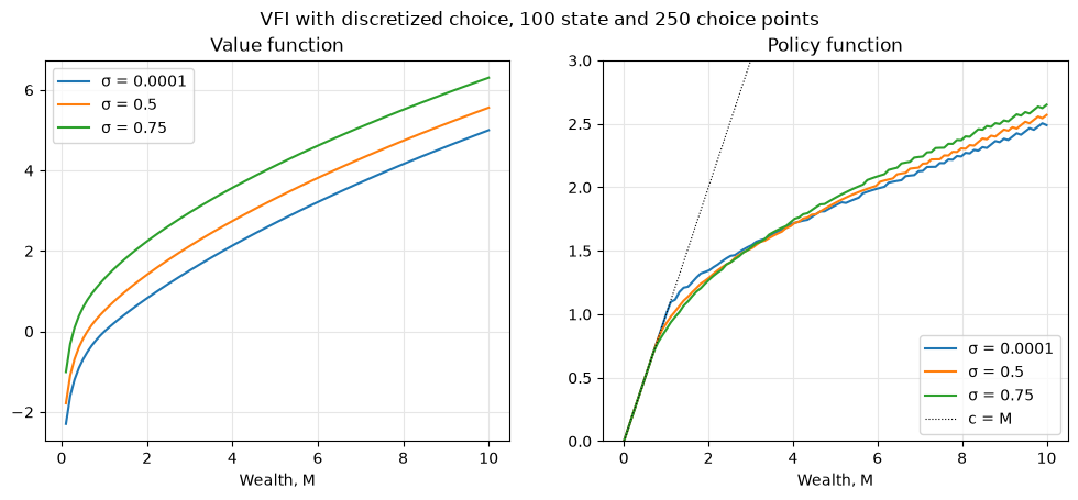

The consumer eats all wealth up to a threshold and saves a part of it above. With more income risk the threshold is lower and consumption at low wealth is smaller: the consumer saves for precaution. At high wealth the order flips, because with $\log\tilde y \sim N(0,\sigma^2)$ a larger $\sigma$ also raises mean income $\exp(\sigma^2/2)$ , which is also why the value function is higher.

Happy with the accuracy of the solution?
How would you change the model to vary the risk while keeping mean income fixed?

VFI with continuous choice¶

The second approach drops the choice grid and solves the maximization in the Bellman equation numerically in every state:

c_i(M_j) = \arg\max_{0 \leqslant c \leqslant M_j} \Big\{ u(c) + \beta \sum_k \omega_k\, \hat V_{i-1}\big(R(M_j - c) + y_k\big) \Big\}

the choice is no longer restricted to a grid, so the policy can be much more accurate
but every iteration runs an optimizer in every state, which is slow
the problem is bounded, so the optimizer must handle the constraint, and Newton is not an option because $\hat V$ is only piecewise linear

scipy.optimize.minimize_scalar with method='bounded' runs Brent’s method on an interval, combining golden section search with parabolic interpolation, without derivatives. See the link in the bottom of the page to the visualization of the method by Oscar Fernandez.

def bellman_continuous(m, V0):
    '''Bellman operator with continuous choice, solved by Brent's method in every state'''
    def minus_maximand(c, M):
        EV = interp(m.next_wealth(M, c, m.quadp), m.grid, V0) @ m.quadw
        return -(m.u(c) + m.beta * EV)                    # minus: minimize_scalar minimizes
    V1, c1 = np.empty(m.ngrid), np.empty(m.ngrid)
    for j, M in enumerate(m.grid):
        if M <= m.grid[0]:
            c1[j] = M                                     # no room to optimize at the first point
        else:
            res = minimize_scalar(minus_maximand, args=(M,), method='bounded',
                                  bounds=(m.eps, M), options={'xatol': 1e-10})
            c1[j] = res.x
        V1[j] = -minus_maximand(c1[j], M)
    return V1, c1

fig, (ax1, ax2) = plt.subplots(1, 2, figsize=(12, 4.5))
for sigma in (0.0001, 0.5, 0.75):
    ms = deaton(sigma=sigma)
    last = {}                                             # the callback keeps the last iteration
    c = solve_vfi(ms, bellman_continuous, callback=lambda **kw: last.update(kw))
    ax1.plot(ms.grid[1:], last['value'][1:], label=f'σ = {sigma}')
    ax2.plot(ms.grid, c, label=f'σ = {sigma}')
ax2.plot(ms.grid, ms.grid, 'k:', lw=0.8, label='c = M')
ax2.set(ylim=(0, 3))
for ax, t in ((ax1, 'Value function'), (ax2, 'Policy function')):
    ax.set(xlabel='Wealth, M', title=t)
    ax.grid(color='0.9')
    ax.legend()
fig.suptitle('VFI with truly continuous choice, 100 state and 250 choice points')
plt.show()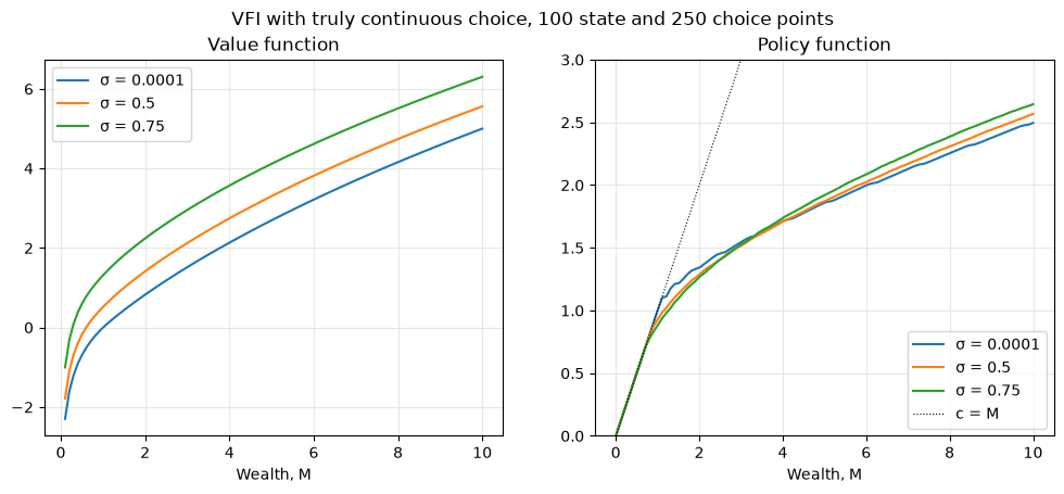

Happy with the accuracy of the solution?
What contributes to the inaccuracy of the solution now?

Time iterations on the Euler equation¶

The third approach does not use the value function at all. The Euler equation holds for the optimal policy, so given a policy $c_{i-1}$ for next period, the policy for this period solves, in every state $M_j$

u'(c) = \beta R \sum_k \omega_k\, u'\Big(c_{i-1}\big(R(M_j - c) + y_k\big)\Big)

for $c$ , a root-finding problem in one variable.

If the residual $u'(c) - \beta R\, \mathbb{E}\, u'(c')$ is still positive at $c = M_j$ , the borrowing constraint binds and $c = M_j$ .

Iterating this operator, the time iterations, converges to the optimal policy.

def euler_residual(m, c, M, c0):
    '''LHS - RHS of the Euler equation at (M, c), with next period policy c0 on the grid'''
    M1 = m.next_wealth(np.atleast_1d(M)[:, None], np.atleast_1d(c)[:, None], m.quadp[None, :])
    c1 = np.maximum(interp(M1, m.grid, c0), m.eps)        # next period consumption, kept positive
    return 1 / c - m.beta * m.R * ((1 / c1) @ m.quadw).squeeze()   # marginal utility u'(c) = 1/c

def solve_timeiter(m, maxiter=500, tol=1e-4, callback=None):
    '''Time iterations: solve the Euler equation for c in every state, returns the policy'''
    c0 = m.grid.copy()                                    # start from consuming everything
    for i in range(maxiter):
        c1 = np.empty(m.ngrid)
        for j, M in enumerate(m.grid):
            if M <= m.grid[0] or euler_residual(m, M, M, c0) > 0:
                c1[j] = M                                 # constraint binds: consume everything
            else:
                c1[j] = brentq(lambda c: euler_residual(m, c, M, c0), m.eps, M, xtol=1e-12)
        err = np.max(np.abs(c1 - c0))
        if callback: callback(iter=i, policy=c1, err=err)
        if err < tol: break
        c0 = c1
    else:
        raise RuntimeError('No convergence: maximum number of iterations achieved')
    return c1

fig, (ax1, ax2) = plt.subplots(1, 2, figsize=(12, 4.5))
for sigma in (0.0001, 0.5, 0.75):
    ms = deaton(sigma=sigma)
    last = {}                                             # the callback keeps the last iteration
    c = solve_timeiter(ms, callback=lambda **kw: last.update(kw))
    ax2.plot(ms.grid, c, label=f'σ = {sigma}')
ax2.plot(ms.grid, ms.grid, 'k:', lw=0.8, label='c = M')
ax2.set(ylim=(0, 3))
for ax, t in ((ax1, 'Value function'), (ax2, 'Policy function')):
    ax.set(xlabel='Wealth, M', title=t)
    ax.grid(color='0.9')
ax2.legend()
fig.suptitle('Time iterations, 100 state and 250 choice points')
plt.show()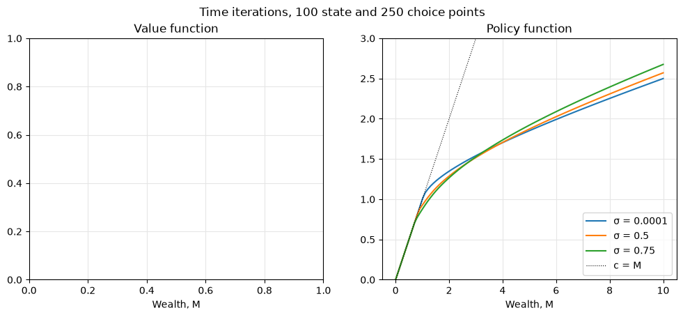

Happy with the accuracy of the solution?
What contributes to it now?

Accuracy: the Euler equation residuals¶

The Euler equation residual of Class 15 measures the error of a numerical solution at an arbitrary point, now with the expectation over income computed by quadrature:

\varepsilon(M) = \frac{u'\big(c(M)\big) - \beta R\, \mathbb{E}_y\, u'\Big(c\big(R(M - c(M)) + \tilde y\big)\Big)}{u'\big(c(M)\big)}

The residual is relative, so it reads as a fraction of the marginal utility. It is evaluated on a dense grid, ten times finer than the solver’s, with the policy interpolated, and only where the constraint does not bind.

Time iterations are the most accurate, because they solve the very equation the residual measures, up to the interpolation of next period’s policy. VFI with continuous choice comes next and VFI with discretized choice last.

Where it breaks: the definition of a corner solution. The bounded optimizer of bellman_continuous cannot land exactly on the bound $c = M$ , it stops a hair below. A corner test with an absolute tolerance, c < M - 1e-10, then counts the corners as interior points, where the residual is large by construction, and the measured error of the continuous solver is twenty times too big. The relative tolerance rtol in the code below removes them. Every accuracy measure needs this kind of care.

Simulation and Keane’s test¶

The simulator draws income from its true distribution, not from the quadrature nodes, and applies the interpolated policy, capped at the available wealth.

def simulate(m, c, M0, T=50, seed=None):
    '''Simulate T periods from initial wealth M0 (scalar or array) with the policy c on the grid'''
    rng = np.random.default_rng(seed)
    M0 = np.atleast_1d(M0).astype(float)
    M, C = np.empty((M0.size, T)), np.empty((M0.size, T))
    M[:, 0] = M0
    for t in range(T):
        C[:, t] = np.minimum(interp(M[:, t], m.grid, c), M[:, t])   # no borrowing
        if t < T - 1:
            y = lognorm.rvs(m.sigma, size=M0.size, random_state=rng)
            M[:, t + 1] = m.next_wealth(M[:, t], C[:, t], y)
    return M, C

Keane’s test needs the deterministic model with $\beta R = 1$ . A log-normal income with a tiny $\sigma$ puts all quadrature nodes at $y = 1$ , so the same code covers it. Consumption simulated from $M_0 = 5$ should stay at $c^\star = ((R-1) M_0 + 1)/R$ forever.

k = deaton(beta=0.9, R=1/0.9, sigma=1e-10, nquad=2)       # deterministic income y = 1, beta*R = 1
M0, T = 5.0, 100
cstar = ((k.R - 1) * M0 + 1) / k.R
fig, ax = plt.subplots(figsize=(10, 4))
for name, solver in (('VFI, discretized choice', lambda: solve_vfi(k, bellman_discretized, tol=1e-8, maxiter=2000)),
                     ('VFI, continuous choice', lambda: solve_vfi(k, bellman_continuous, tol=1e-8, maxiter=2000)),
                     ('time iterations', lambda: solve_timeiter(k, tol=1e-10, maxiter=2000))):
    _, C = simulate(k, solver(), M0, T)
    ax.plot(C[0], label=name)
    print(f'{name:<25} max |c_t / c* - 1| = {np.max(np.abs(C[0] / cstar - 1)):.1e}')
ax.axhline(cstar, c='k', lw=0.8, ls=':', label='c*')
ax.set(xlabel='period', ylabel='simulated consumption', title="Keane's test")
ax.grid(color='0.9'); ax.legend()
plt.show()

VFI, discretized choice   max |c_t / c* - 1| = 1.4e-02

VFI, continuous choice    max |c_t / c* - 1| = 5.3e-08

time iterations           max |c_t / c* - 1| = 2.7e-09

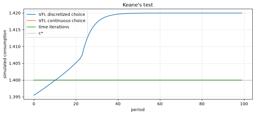
The discretized solver fails the test, with consumption off by about one percent and drifting, while the other two keep it flat to seven digits or better.

Speed and accuracy compared¶

The Euler residual of a policy, on a dense grid and at the interior points only:

def accuracy(m, c, factor=10, rtol=1e-6):
    '''Mean absolute relative Euler residual of the policy c on a dense grid, interior points only'''
    M = np.linspace(m.grid[1], m.Mbar, m.ngrid * factor)  # dense grid, first point skipped
    cM = interp(M, m.grid, c)                             # interpolated policy
    er = euler_residual(m, cM, M, c) * cM                 # relative Euler residual, divided by u'(c) = 1/c
    interior = cM < M * (1 - rtol)                        # drop the corner solutions c = M
    return np.mean(np.abs(er[interior]))

Each solver now runs for the three values of $\sigma$ and for a growing state grid, with the choice grid of the discretized solver fixed at 250 points. The solvers stop at a tight tolerance, 10^-8, so that what we measure is the error of the grid and not of the stopping rule. For $\sigma$ near zero the model is set to $\beta R = 1$ , where Keane’s test applies; for the other two values of $\sigma$ it does not.

solvers = {'VFI, discretized choice': lambda m: solve_vfi(m, bellman_discretized, tol=1e-8, maxiter=2000),
           'VFI, continuous choice': lambda m: solve_vfi(m, bellman_continuous, tol=1e-8, maxiter=2000),
           'time iterations': lambda m: solve_timeiter(m, tol=1e-8, maxiter=2000)}
sigmas, grids = (0.0001, 0.5, 0.75), (50, 100, 200, 400)
M0, T = 5.0, 100                                          # Keane's test: initial wealth and periods
fig, axes = plt.subplots(3, 3, figsize=(15, 12))
for row, sigma in zip(axes, sigmas):
    keane_test = sigma < 0.01                             # sigma near zero: Keane's test with beta*R = 1
    for name, solve in solvers.items():
        keane, euler, runtime = [], [], []
        for n in grids:
            if keane_test:
                m = deaton(sigma=sigma, R=1/0.9, nquad=2, ngrid=n)   # beta = 0.9, so beta*R = 1
            else:
                m = deaton(sigma=sigma, ngrid=n)
            t0 = time.perf_counter()
            c = solve(m)
            runtime.append(time.perf_counter() - t0)
            euler.append(accuracy(m, c))
            if keane_test:
                _, C = simulate(m, c, M0, T, seed=2026)
                cstar = ((m.R - 1) * M0 + 1) / m.R
                keane.append(np.max(np.abs(C[0] / cstar - 1)))
        if keane_test:
            row[0].plot(grids, keane, 'o-', label=name)
        row[1].plot(grids, euler, 'o-', label=name)
        row[2].plot(grids, runtime, 'o-', label=name)
    if not keane_test:
        row[0].axis('off')
        row[0].text(0.5, 0.5, f"σ = {sigma}\nKeane's test needs σ ≈ 0 and βR = 1",
                    ha='center', va='center', transform=row[0].transAxes)
    titles = ("Keane's test, max |c_t / c* - 1|", 'Mean |Euler residual|', 'Run time, s')
    for ax, t in zip(row, titles):
        ax.set(xscale='log', yscale='log', xlabel='State grid points',
               title=f'{t}, σ = {sigma}' + (', βR = 1' if keane_test else ''))
        ax.set_xticks(grids, [str(n) for n in grids])
        ax.grid(color='0.9')
axes[0, 0].legend()
fig.tight_layout()
plt.show()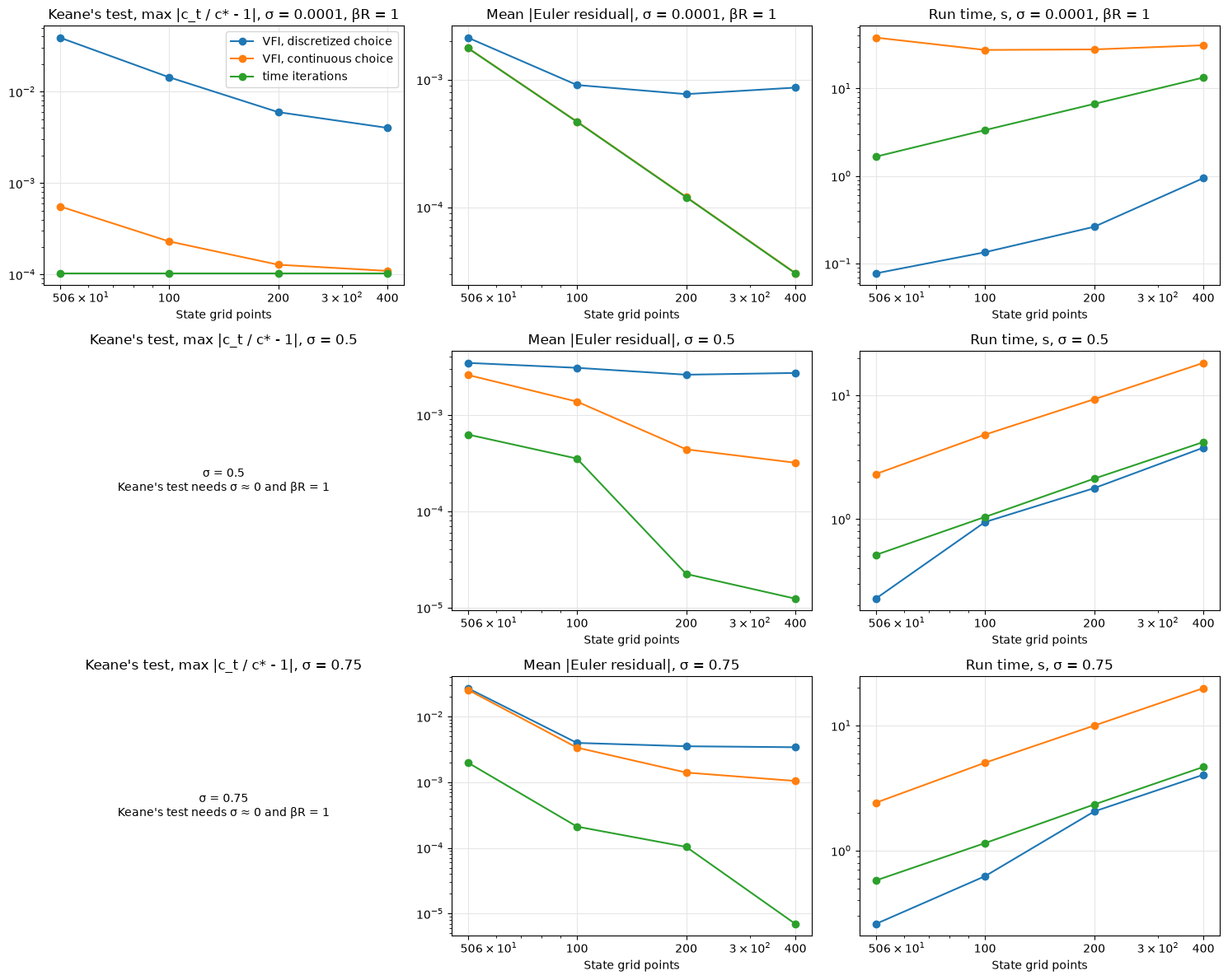

Keane’s test at $\sigma \approx 0$ : the discretized solver fails it at every grid size, off by 4% with 50 points and still by 0.4% with 400, because the choice grid pins consumption only to the nearest share. Time iterations keep consumption within 10^-4 of $c^\star$ at every grid size, which is about as close as a test with $\sigma = 10^{-4}$ can show: the income shocks themselves move consumption by that much over 100 periods. VFI with continuous choice gets there only with 400 points, from $6 \cdot 10^{-4}$ with 50.
Euler residuals: VFI with continuous choice and time iterations improve steadily with the grid. With $\sigma \approx 0$ they are almost identical and fall fourfold for every doubling of the grid, the $h^2$ rate of linear interpolation. With income risk time iterations are well ahead, at about 10^-5 with 400 points. The discretized solver stalls between 10^-3 and $3 \cdot 10^{-3}$ , capped by its choice grid.
Run time: the discretized solver is the fastest without income risk. With risk, time iterations are faster at every grid size and the gap grows with the grid, because each iteration of the discretized solver evaluates every combination of state, choice and quadrature node. Optimizing over a continuous choice in every state is the slowest throughout.

Time iterations are the best of the three: as accurate as VFI with continuous choice or better, and several times faster. A root of the Euler equation is easier to find than a maximum of the Bellman equation, and the Euler equation needs no value function.

Important idea: not using value function is beneficial! (See next lecture)

Why do time iterations not need a value function, and what is lost without one?
Which of the three solvers would still work if the utility function were not concave, or if there were a discrete choice on top of consumption?

References¶

Deaton, A. (1991). Saving and Liquidity Constraints. Econometrica, 59(5), 1221–1248. 10.2307/2938366
Judd, K. L. (1998). Numerical Methods in Economics (p. 633). MIT Press. https://mitpress.mit.edu/9780262100717/numerical-methods-in-economics/