The logit model is the workhorse of the whole course: every dynamic discrete choice model we solve and estimate later has a logit formula at its core, evaluated millions of times inside a fixed point iteration nested inside a likelihood maximization.
Today we build the static logit model in code and, along the way, set up the boilerplate that every model in the course will reuse.
We should know the theory behind the folmulas
We should know how to compute it so that it does not silently produce
nanon the fifth iteration of estimation loop
Running the code for this lecture
The code for this class is in the folder session06-sep10/ of the course code
repository. Today is a practical, so that folder holds the pre-code skeleton we fill
in together, and the completed version appears there afterwards.
You should have cloned that repository already — if not, the instructions are in the algorithms and complexity lecture.
Update your copy before the class. Editing a file in place makes git pull refuse to
update it, so discard whatever you changed while experimenting:
cd sb-dse-code
git reset --hard HEAD
git pull
Nothing in this repository is submitted, so experiment freely — but copy anything you want to keep out of it first, or commit that to a branch of your own.
Setting up the Python environment is covered in Python.
Background on static discrete choice
Deterministic model: the levels and scale do not matter
A decision maker (DM) in state picks from a finite set to maximize :
Two implications, used below for identification and, immediately, for numerics.
Only differences in utilities matter — adding a constant changes nothing:
one alternative’s utility has to be normalized, say to zero
an attribute of the DM are identical across alternatives cannot enter additively separably, only non-linearly, i.e. through cross-effects with attributes of choice
The scale of utility is irrelevant — multiplying by a positive constant changes nothing:
when we add an additively separable random component to the utility, its scale has to be normalized
the variance of the random component is a normalization, not a parameter
it returns below as the scale parameter
Probabilistic choice
Now assume that the DM has private information that the econometrician does not observe, and assume that it enters additively separably in the utility:
The object of interest is then conditional choice probability (CCP)
where is the indicator function and the density of given .
This is the random utility model (RUM) as we know it.
Luce’s own statement is equivalent — with the probability of choosing over and , he required
so the relative odds of two alternatives do not depend on what else is available.
The logit structure thus comes out with no distributional assumption anywhere, and without specifying at all.
Extreme value distribution and max-stability
Luce’s structure comes out of a RUM when the unobserved components have the type I extreme value (Gumbel) distribution:
| Notation | EV1(,) |
|---|---|
| Parameters | Location , scale |
| CDF | |
| Support | |
| Expectation | |
| Mode | |
| Variance | |
| Standard normalization |
where
is the Euler–Mascheroni constant (np.euler_gamma).
Source
import numpy as np
import matplotlib.pyplot as plt
plt.rcParams['figure.figsize'] = [9, 4]

x = np.linspace(-4, 8, 500)
ev1_pdf = lambda x, mu=0., s=1.: np.exp(-(x-mu)/s - np.exp(-(x-mu)/s))/s
fig, ax = plt.subplots()
for mu, s, c in [(0., 1., '#1A6D91'), (2., 1., '#0E8A27'), (0., 2., '#CB1515')]:
    ax.plot(x, ev1_pdf(x, mu, s), lw=2, color=c, label=f'EV1($\\mu$={mu:g}, $\\sigma$={s:g})')
ax.legend(frameon=False)
ax.set_title('Type I extreme value (Gumbel) density')
ax.grid(True, alpha=.3)
plt.show()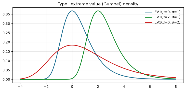
developed to describe the maxima of independent draws — the highest level of a river, the strongest earthquake in a century
extreme value theory gives exactly three limiting distributions of maxima, hence “type I”
The other types are Fréchet (type II) and Weibull (type III)
max-stability, the property we need: the maximum of independent EV1 variables with a common scale is again EV1, with that same scale
For independent with CDFs , , and for the product telescopes:
so the maximum is EV1 with the same scale and location
This is the logsum formula which describes the expected maximum of independent EV1 variables:
Worth confirming once rather than believing:
rng = np.random.default_rng(42)
mu, sigma, n = np.array([0., 1., 2.5]), 1.5, 500_000
draws = mu + sigma * rng.gumbel(size=(n, mu.size))   # EV1(mu_i, sigma), independent
mx = draws.max(axis=1)                               # the maximum over alternatives
mu_max = sigma * np.log(np.sum(np.exp(mu/sigma)))    # logsum formula
print(f'simulated mean of the max = {mx.mean():.4f}')
print(f'logsum + sigma*gamma      = {mu_max + sigma*np.euler_gamma:.4f}')
print(f'simulated variance        = {mx.var():.4f}   theory = {sigma**2*np.pi**2/6:.4f}')
simulated mean of the max = 4.0276
logsum + sigma*gamma = 4.0297
simulated variance = 3.6895 theory = 3.7011
The logit choice probabilities
Marschak (1960): Luce’s structure obtains in a RUM whose are i.i.d. EV1 across alternatives,
independence across alternatives is the whole assumption
location and scale are free: is EV1(0,1) whenever is EV1, and by points 1 and 2 above shifting and scaling utilities changes no choice
The direct derivation — condition on , use max-stability for the rest, then substitute — is in the reading. The general route for any RUM:
the differentiated object is McFadden’s social surplus function McFadden, 1981
the proof: differentiation passes under the integral, and the derivative of a max is the indicator of the argmax
For EV1(0,1) the expected maximum is the logsum, and one line of calculus gives the multinomial logit choice probability:
Keeping instead of normalizing it away — which we want in models with non-linear utility — the same derivation yields
: every exponent goes to zero, , choice is uniformly random
: the probabilities collapse onto the deterministic rule
both limits are numerically nasty, and we meet them again below
and sums to one exactly — the two things we assert in the code
The price of IIA
IIA is an axiom about behavior, and behavior does not always oblige.
The culprit is independence of across alternatives, plainly wrong when two alternatives differ only in paint. Remedies, in increasing computational cost:
Nested / GEV logit — relaxes the substitution pattern, keeps closed forms for the probabilities and the social surplus. The generating function gives multinomial logit, a nested sum of powers gives nested logit McFadden, 1981
Mixed logit — integrates over a distribution of taste coefficients; approximates any RUM, at the cost of simulating the integral
Probit — joint normal errors, rich covariance, no closed form, multidimensional integration
Dynamics — IIA on flow utilities does not carry over to alternative-specific values, because continuation values differ. One reason we tolerate EV1 all course
The scale parameter is a normalization in a linear-utility model. Why is it not a normalization once utility is non-linear in parameters?
Numerical issues: three formulas and how they break
Everything above reduces to three expressions that our code has to evaluate, over and over, inside solvers and likelihoods:
Mathematically they are innocuous. On a computer they are not, because exp is the
fastest way to leave the range of a floating point number.
Exponentiation is dangerous
Do you expect the following code to run without errors? What will it print?
a = 2.
for i in range(14):
    print(f'i={i:2d}   a={a:.3e}   exp(a)={np.exp(a):.3e}')
    a **= 1.25
Output
i= 0   a=2.000e+00   exp(a)=7.389e+00
i= 1   a=2.378e+00   exp(a)=1.079e+01
i= 2   a=2.954e+00   exp(a)=1.918e+01
i= 3   a=3.872e+00   exp(a)=4.804e+01
i= 4   a=5.432e+00   exp(a)=2.285e+02
i= 5   a=8.292e+00   exp(a)=3.993e+03
i= 6   a=1.407e+01   exp(a)=1.292e+06
i= 7   a=2.725e+01   exp(a)=6.856e+11
i= 8   a=6.227e+01   exp(a)=1.105e+27
i= 9   a=1.749e+02   exp(a)=9.297e+75
i=10   a=6.362e+02   exp(a)=1.892e+276
i=11   a=3.195e+03   exp(a)=inf
i=12   a=2.402e+04   exp(a)=inf
i=13   a=2.990e+05   exp(a)=inf
/tmp/ipykernel_4047/1817667625.py:3: RuntimeWarning: overflow encountered in exp
  print(f'i={i:2d}   a={a:.3e}   exp(a)={np.exp(a):.3e}')
IEEE 754 double precision runs out
at about , so np.exp overflows to inf as soon as its argument
exceeds
print(f'largest double      = {np.finfo(float).max:.6e}')
print(f'log of it           = {np.log(np.finfo(float).max):.6f}')
print(f'smallest normal     = {np.finfo(float).tiny:.6e}')
print(f'log of it           = {np.log(np.finfo(float).tiny):.6f}')
largest double = 1.797693e+308
log of it = 709.782713
smallest normal = 2.225074e-308
log of it = -708.396419
So utilities above roughly 709 overflow and utilities below roughly -745 underflow to
zero. That sounds like a lot of utility until you remember that we divide by ,
that in a dynamic model is a discounted lifetime value with , and
that an optimizer exploring the parameter space will happily try on its
way to somewhere sensible. A single inf turns into inf/inf = nan, and nan
propagates silently through the whole fixed point.
def logit_naive(v, sigma=1.0, axis=0):
    '''Logit choice probabilities, straight from the formula'''
    e = np.exp(np.asarray(v)/sigma)
    return e/e.sum(axis=axis, keepdims=True)

v = np.array([1000., 1001., 999.])       # utility differences are just 1 and 2
with np.errstate(over='ignore', invalid='ignore'):
    print('naive :', logit_naive(v))
naive : [nan nan nan]
De-maxing
The fix follows from the fact that only utility differences matter. For any constant ,
because cancels from numerator and denominator. Choosing means we only ever exponentiate non-positive numbers, so the largest term is exactly 1 and overflow is impossible. Underflow may still happen, but it replaces a astronomically small number by exactly zero, which is harmless — and the denominator is at least 1, so we never divide by zero.
The same trick applies to the logsum, where the constant is added back afterwards:
def logit(v, sigma=1.0, axis=0):
    '''Logit choice probabilities, computed with de-maxing.
    Alternatives along the given axis, any other dimensions are states.
    '''
    v = np.asarray(v, dtype=float)/sigma
    mx = np.max(v, axis=axis, keepdims=True)      # de-maxing constant
    e = np.exp(v - mx)                            # exponent of non-positive numbers
    return e/e.sum(axis=axis, keepdims=True)

def logsum(v, sigma=1.0, axis=0):
    '''Log-sum-exp = expected maximum of v + EV1 shocks, up to sigma*gamma'''
    v = np.asarray(v, dtype=float)/sigma
    mx = np.max(v, axis=axis, keepdims=True)
    ls = mx + np.log(np.sum(np.exp(v - mx), axis=axis, keepdims=True))
    return sigma*np.squeeze(ls, axis=axis)

print('de-maxed :', logit(v))
print('logsum   :', logsum(v))
print('naive:', np.log(np.sum(np.exp(v))))
de-maxed : [0.24472847 0.66524096 0.09003057]
logsum : 1001.4076059644444
naive: inf
/tmp/ipykernel_4047/1859438880.py:19: RuntimeWarning: overflow encountered in exp
  print('naive:', np.log(np.sum(np.exp(v))))
The de-maxed version returns the same numbers a hand calculation would: utility differences of 1 and 2 give probabilities regardless of the level 1000.
Never take the log of a probability
The log-likelihood needs , and the obvious np.log(logit(v)) is a bad idea:
when a probability underflows to zero — which it will, for a badly-fitting parameter
guess or a small — the log is and the optimizer is handed a wall
instead of a gradient. Compute log-probabilities directly instead, where the subtraction
happens before any exponentiation can destroy information:
def loglogit(v, sigma=1.0, axis=0):
    '''Log of the logit choice probabilities, without ever taking log of a probability'''
    v = np.asarray(v, dtype=float)
    return (v - np.expand_dims(logsum(v, sigma, axis), axis))/sigma

w = np.array([0., -40., -900.])            # third alternative is hopeless
with np.errstate(divide='ignore'):
    print('log(logit(w)) :', np.log(logit(w)))
print('loglogit(w)   :', loglogit(w))
log(logit(w)) : [ 0. -40. -inf]
loglogit(w) : [ 0. -40. -900.]
The third alternative has log-probability -900, not : a small number that a likelihood can work with, rather than a missing value that stops the optimizer.
The scale parameter is a numerical hazard
Dividing by before de-maxing is what keeps small usable. As the scaled utilities diverge, but their differences after de-maxing stay finite or underflow gracefully to zero.
u = np.array([1.0, 1.5, 0.8])
for s in [10., 1., 0.1, 1e-3, 1e-8]:
    with np.errstate(over='ignore', invalid='ignore'):
        naive = logit_naive(u, sigma=s)
    print(f'sigma={s:<8g} naive={np.array2string(naive, precision=3)}'
          f'   de-maxed={np.array2string(logit(u, sigma=s), precision=3)}')
sigma=10 naive=[0.33 0.347 0.323] de-maxed=[0.33 0.347 0.323]
sigma=1 naive=[0.288 0.475 0.236] de-maxed=[0.288 0.475 0.236]
sigma=0.1 naive=[6.687e-03 9.924e-01 9.050e-04] de-maxed=[6.687e-03 9.924e-01 9.050e-04]
sigma=0.001 naive=[nan nan nan] de-maxed=[7.125e-218 1.000e+000 9.860e-305]
sigma=1e-08 naive=[nan nan nan] de-maxed=[0. 1. 0.]
At the naive formula is already nan, while the de-maxed one reports
the deterministic choice, which is the correct limit. Note also what the de-maxed answer
does not do: it never returns a probability outside , and the row still sums to
one, which is the check to write into the code.
p = logit(np.array([[1., 2.], [3., 0.], [-2., 5.]]), sigma=0.4)   # 3 alternatives x 2 states
print(p, end='\n\n')
assert np.allclose(p.sum(axis=0), 1.0), 'choice probabilities must sum to one'
assert np.all(p >= 0.), 'choice probabilities must be non-negative'
print('sums over alternatives:', p.sum(axis=0))
[[6.69282615e-03 5.52776578e-04]
[9.93303472e-01 3.72457929e-06]
[3.70169754e-06 9.99443499e-01]]
sums over alternatives: [1. 1.]
Logit as a smoothing device
There is a second reason to have this machinery at hand, unrelated to discrete choice: the logsum is a smooth maximum, and the logit probability is a smooth indicator. Many objects in structural models are kinked or discontinuous — progressive tax schedules, eligibility thresholds, the upper envelope of value functions in discrete-continuous choice Iskhakov et al., 2017, the likelihood correspondence in games with multiple equilibria — and a solver that needs derivatives cannot cope with them.
For two functions and , the kinked is approximated by
and the approximation error is uniformly bounded and known. Since is monotone,
If this collapses to , and symmetrically otherwise, with the bound 2 attained exactly where . Hence
so the error is controlled by choosing — and note that this is the same that has an economic interpretation as the scale of the taste shocks. Smoothing a kink and adding an EV1 shock are the same operation.
Source
x = np.linspace(-2, 4, 1000)
f1 = 2 * np.exp(-0.5 * (x - 0.5)**2) + 0.3 * x**2 - 1
f2 = -0.4 * x**3 + 1.2 * x**2 + 0.5 * x + 0.5 + 0.3 * np.sin(2*x) - 0.5
f3 = lambda s: s * np.log(np.exp(f1/s) + np.exp(f2/s))
fig, ax = plt.subplots(figsize=(10, 6), dpi=100)
ax.plot(x, f1, linewidth=2.0, color="#1A6D91", label='f(x)', alpha=0.8)
ax.plot(x, f2, linewidth=2.0, color="#0E8A27", label='g(x)', alpha=0.8)
ax.legend(frameon=True, loc='lower left')
s1, s2 = 0.02, 0.8
for s in np.linspace(s1, s2, 10):
    ax.plot(x, f3(s), linewidth=1.0, color="#CB1515", alpha=1 - s)
ax.set_title(f'Smoothed maximum of two functions, sigma from {s2:0.2f} down to {s1:0.2f}', fontsize=14, pad=20)
ax.grid(True, alpha=0.3, linestyle='-', linewidth=0.5)
ax.set_xlim(-2, 4); ax.set_ylim(-1, 4)
plt.show()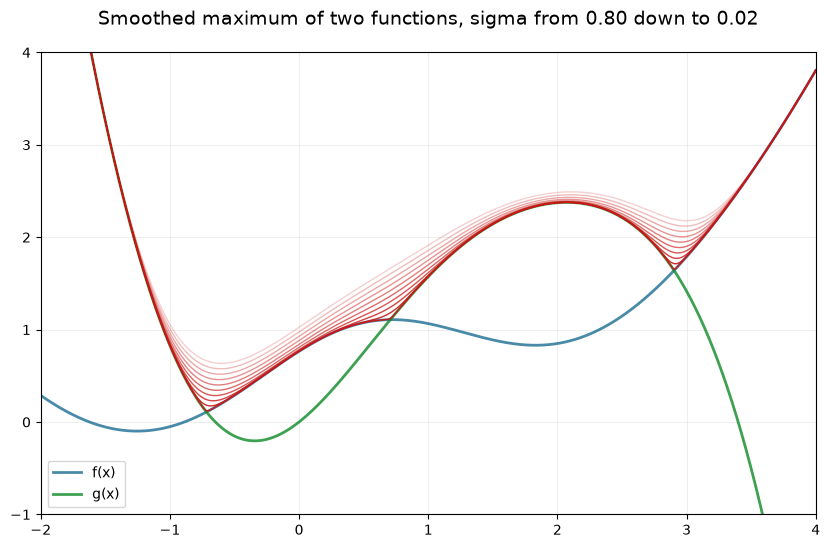
Note that the plot above is computed with the naive np.exp(f1/s), which is fine at
for functions of order one and starts overflowing well before
. The de-maxed logsum written above handles the whole range — a good
first exercise in the practical.
A jump is smoothed by the logit probability rather than the logsum. If is smooth except for a jump of size at ,
where . Convergence here is only pointwise, not uniform: at itself the smoothed function is off by no matter how small is.
Source
x0 = 0.25
x = np.linspace(-1, 2, 10000)
g1 = lambda x: -0.4 * x**3 + 1.2 * x**2 + 0.5 * x + 0.5 + 0.3 * np.sin(2*x) - 0.5
g2 = lambda x: 2 * np.exp(-0.5 * (x - 0.5)**2) + 0.3 * x**2 - 1
fd = (x < x0)*g1(x) + (x > x0)*g2(x)
ix = np.max(np.where(x <= x0))
gap = g2(x[ix]) - g1(x[ix])
fd[ix] = np.nan                                   # to show the discontinuity
smooth = lambda x, s: fd + gap*(1/(1 + np.exp(-(x - x0)/s)) - (x > x0))
fig, ax = plt.subplots(figsize=(10, 6), dpi=100)
ax.plot(x, fd, linewidth=2.0, color="#2355A1", label='f(x)')
ax.legend(frameon=True, loc='lower left')
s1, s2 = 0.005, 0.1
for s in np.linspace(s1, s2, 10):
    ax.plot(x, smooth(x, s), linewidth=1.0, color="#CB1515", alpha=1 - 8*s)
ax.set_title(f'Smoothed discontinuity, sigma from {s2:0.3f} down to {s1:0.3f}', fontsize=14, pad=20)
ax.grid(True, alpha=0.3, linestyle='-', linewidth=0.5)
ax.set_xlim(-1, 2); ax.set_ylim(-1, 2)
plt.show()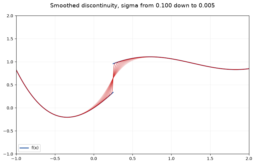
The model we build today
The point of the practical is not the logit formula itself — it is one line — but the shape of the code around it. Every structural project in this course, and your own project later in the semester, has the same six parts:
a model object holding the parameters, with the “model parts” (utility, transitions) attached to it
a solver that maps parameters into the model solution
a simulator that generates data from a solved model
a graphical module that shows what the model and the data look like
an estimator that recovers parameters from data (from the NFXP class onwards)
a counterfactual simulator that changes something and re-solves (later still)
Keep these separate from the run scripts that call them. A run script is throwaway; the model, solver and simulator are what you reuse for the whole semester.
Specification
A decision maker in state chooses one of alternatives, each described by a vector of attributes. We consider two utility specifications:
Linear:
Log:
with state-dependent coefficients tied together as and , so the vector of structural parameters is plus the scale . Choice probabilities are logit with scale , as derived above.
The state enters only through the coefficients here, which is deliberately minimal — enough to have something to compare across states, and few enough parameters that the dashboard is readable.
The model object
Start with what holds the parameters. Two details are worth the extra lines: __str__,
so that printing a model tells you what it is, and __setattr__, so that an
inconsistent model cannot be created in the first place. Shape bugs found at assignment
time cost minutes; the same bug found inside a likelihood costs an afternoon.
class model:
    '''Static random utility model with EV1 taste shocks'''

    def __init__(self,
                 label='noname',
                 nalt=5,                    # number of alternatives
                 nattr=3,                   # number of attributes of each alternative
                 attr=None,                 # attribute values Y, (nalt, nattr)
                 param=None,                # structural parameters beta, (nattr,)
                 st=np.array([1, 2]),       # states of the decision maker
                 util_type='linear',        # 'linear' or 'log'
                 sigma=1.0):                # scale of the taste shocks
        self.label = label
        self.nalt = nalt                    # dimensions first: __setattr__ checks against them
        self.nattr = nattr
        self.st = st
        self.util_type = util_type
        self.sigma = sigma
        self.attr = np.ones((nalt, nattr)) if attr is None else attr
        self.param = np.zeros(nattr) if param is None else param

    def __str__(self):
        '''Human readable representation of the model'''
        return (f'Model "{self.label}" [{self.util_type}]: {self.nalt} alternatives, '
                f'{self.nattr} attributes, {self.st.size} states, sigma={self.sigma:g}\n'
                f'  beta = {np.array2string(self.param, precision=3, separator=", ")}')

    def __setattr__(self, name, value):
        '''Check consistency of the model attributes on assignment'''
        if name == 'attr':
            value = np.asarray(value, dtype=float)
            assert value.shape == (self.nalt, self.nattr), \
                f'attr must have shape ({self.nalt}, {self.nattr}), got {value.shape}'
        if name == 'param':
            value = np.asarray(value, dtype=float)
            assert value.size == self.nattr, \
                f'param must have {self.nattr} elements, got {value.size}'
        if name == 'sigma':
            assert value > 0, 'sigma must be strictly positive'
        super().__setattr__(name, value)

    # ---- model parts ----

    def beta_coef(self):
        '''State-specific coefficients, (nattr, nstates)'''
        beta_st = np.empty((self.nattr, self.st.size))
        beta_st[:, 0] = self.param
        beta_st[:, 1] = self.param/2
        return beta_st

    def utility(self):
        '''Deterministic component of utility, (nalt, nstates)'''
        if self.util_type == 'linear':
            return self.attr @ self.beta_coef()
        elif self.util_type == 'log':
            return np.log(self.attr) @ self.beta_coef()
        raise ValueError(f'Unknown utility specification: {self.util_type}')

    def save_solution(self, chpr):
        '''Store the computed choice probabilities in the model object'''
self.solution = chpr__setattr__is called for every assignment, including the ones inside__init__. Why mustself.naltbe set beforeself.attr?What would break if
beta_coefwere computed once in__init__and stored?Where would the transition matrix live in this design, once the model becomes dynamic?
The solver
With logit already written and tested, the solver is three lines. Notice that it both
returns the solution and stores it on the model — convenient for plotting, and the reason
the simulator can assert that the model has been solved.
def model_solve(m):
    '''Solve the model: choice probabilities, alternatives in rows, states in columns'''
    chpr = logit(m.utility(), sigma=m.sigma, axis=0)     # de-maxed, see above
    assert np.allclose(chpr.sum(axis=0), 1.0), 'choice probabilities do not sum to one'
    m.save_solution(chpr)
    return chpr

def model_logsolve(m):
    '''Log choice probabilities, for the likelihood later in the course'''
    return loglogit(m.utility(), sigma=m.sigma, axis=0)
The simulator
Simulating a discrete choice is the inverse-CDF method: form the cumulative
probabilities along the alternatives, draw , and find the interval that
contains it. np.searchsorted does the search in per draw and is
vectorized over draws, which matters when we simulate a hundred thousand agents inside
an MSM criterion later.
import pandas as pd

def model_simulate(m, chpr=None, nobs=10, rng=None):
    '''Simulate nobs decision makers from a solved model, return a pandas DataFrame'''
    assert chpr is not None or hasattr(m, 'solution'), \
        'solve the model first, or pass choice probabilities to the simulator'
    chpr = m.solution if chpr is None else chpr
    rng = np.random.default_rng() if rng is None else rng
    var_names = ['id', 'st', 'choice'] + [f'attr{i}' for i in range(1, m.nattr + 1)]
    data = pd.DataFrame(np.nan, index=range(nobs), columns=var_names)
    data['id'] = 1 + np.arange(nobs)
    data['st'] = rng.integers(m.st.size, size=nobs)          # states drawn uniformly
    cumulative = np.cumsum(chpr, axis=0)                     # cdf over alternatives
    u = rng.random(nobs)                                     # uniform draws
    for st in range(m.st.size):
        mask = data['st'] == st
        # inverse cdf: index of the first cumulative probability exceeding u
        data.loc[mask, 'choice'] = np.searchsorted(cumulative[:, st], u[mask], side='right')
        # attach the attributes of the chosen alternative
        data.loc[mask, var_names[3:]] = m.attr[data.loc[mask, 'choice'].astype(int), :]
    dtypes = [np.int32, np.int32, np.int32] + [np.float64]*m.nattr
    return data.astype(dict(zip(var_names, dtypes)))
Why
side='right'and notside='left'? What happens to a zero-probability alternative under each?The last cumulative probability is 1 only up to floating point. Can
searchsortedreturn an out-of-range index, and what would that do?We draw one uniform per agent. How many draws would the “obvious” alternative — simulating the and taking the argmax — need, and would it give the same answer?
rng = np.random.default_rng(2026)
nalt, nattr = 5, 3
attr = rng.uniform(1, 10, size=(nalt, nattr))
m1 = model(nalt=nalt, nattr=nattr, attr=attr, param=np.array([0.1, 0.35, 0.2]), label='model 1')
print(m1)
model_solve(m1)
simdata = model_simulate(m1, nobs=2500, rng=rng)
simdata.head()
Model "model 1" [linear]: 5 alternatives, 3 attributes, 2 states, sigma=1
beta = [0.1 , 0.35, 0.2 ]
The graphical module
Three plotting functions, each of which can either make its own figure or draw into axes handed to it. That second option is what makes the dashboard possible without duplicating a line of plotting code.
import matplotlib

def plot_attributes(m, ax=None):
    '''Bar plot of the attributes of each alternative'''
    if ax is None:
        fig, ax = plt.subplots(figsize=(6, 4))
    width, x = 0.25, np.arange(m.nalt)
    for i in range(m.nattr):
        ax.bar(x + width*i, m.attr[:, i], width, label=f'attr{i+1}')
    ax.set_ylim(0, ax.get_ylim()[1]*1.15)
    ax.set_title(f'Attributes — {m.label}', fontsize=12)
    ax.set_xlabel('Alternatives')
    ax.legend(loc='upper left', ncols=m.nattr, fontsize=8)

def plot_choice_probabilities(m, ax=None):
    '''Bar plot of the model solution, one panel per state'''
    assert hasattr(m, 'solution'), 'solve the model before plotting its solution'
    if ax is None:
        fig, ax = plt.subplots(1, m.st.size, figsize=(10, 4))
        fig.suptitle(f'Choice probabilities — {m.label}', fontsize=13)
    ymax = 0
    for i in range(min(len(ax), m.st.size)):
        ax[i].bar(range(m.nalt), m.solution[:, i], color='xkcd:fresh green')
        ax[i].set_title(f'State {i}', fontsize=11)
        ax[i].set_xlabel('Alternatives')
        ax[i].set_ylabel('Probability')
        ymax = max(ymax, ax[i].get_ylim()[1])
    for i in range(min(len(ax), m.st.size)):
        ax[i].set_ylim(0, ymax)          # common vertical scale, or the panels lie

def plot_data(m, data, ax=None):
    '''Histograms of simulated choices: pooled, then one panel per state'''
    if ax is None:
        fig, ax = plt.subplots(1, m.st.size + 1, figsize=(12, 4))
        fig.suptitle(f'Frequencies of simulated choices — {m.label}', fontsize=13)
    bins = np.arange(-.5, m.nalt + .5, 1)
    nax, ymax = min(len(ax), m.st.size + 1), 0
    for i in range(nax):
        if i == 0:
            ax[i].hist(data['choice'], bins=bins, edgecolor='white', color='xkcd:light blue')
            ax[i].set_title(f'Pooled, obs={data.shape[0]}', fontsize=11)
        else:
            mask = data['st'] == i - 1
            ax[i].hist(data.loc[mask, 'choice'], bins=bins, edgecolor='white', color='xkcd:pale orange')
            ax[i].set_title(f'State {i-1}, obs={mask.sum()}', fontsize=11)
        ax[i].set_xlabel('Alternatives')
        ax[i].set_ylabel('Frequency')
        ymax = max(ymax, ax[i].get_ylim()[1])
    for i in range(nax):
        ax[i].set_ylim(0, ymax)

def plot_dashboard(m, data):
    '''Attributes and solution on top, simulated data below'''
    ncols = m.st.size + 1
    fig, axs = plt.subplots(2, ncols, figsize=(12, 7), layout='constrained')
    fig.suptitle(f'Dashboard — {m.label}', fontsize=14)
    ax = list(axs.flatten())
    plot_attributes(m, ax=ax[0])
    plot_choice_probabilities(m, ax=ax[1:ncols])
    plot_data(m, data=data, ax=ax[ncols:2*ncols])
Source
plot_dashboard(m1, data=simdata)
plt.show()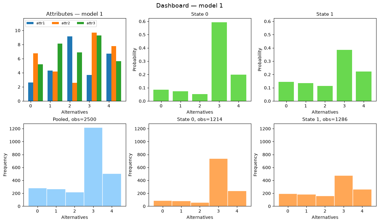
The dashboard is the whole point of building the graphical module: one function call shows the primitives, the solution and the data side by side, so that changing a parameter and re-running gives an immediate read on what that parameter does. This is how you develop intuition about identification — long before writing an estimator, you should be able to say which feature of the data each parameter moves.
Playing with the model
Source
def compare(models, data=None):
    '''Solve several models and put their choice probabilities side by side'''
    fig, axs = plt.subplots(len(models), 2, figsize=(10, 3.2*len(models)), layout='constrained')
    axs = np.atleast_2d(axs)
    for k, m in enumerate(models):
        model_solve(m)
        plot_choice_probabilities(m, ax=list(axs[k]))
        axs[k][0].set_ylabel(f'{m.label}\nProbability')
    plt.show()
The role of . One coefficient moved from 0.1 to 0.9 reshuffles the whole profile of choice probabilities, and does so differently in the two states because shrinks every effect by half.
mA = model(nalt=nalt, nattr=nattr, attr=attr, param=np.array([0.1, 0.35, 0.2]), label='beta1 = 0.1')
mB = model(nalt=nalt, nattr=nattr, attr=attr, param=np.array([0.9, 0.35, 0.2]), label='beta1 = 0.9')
compare([mA, mB])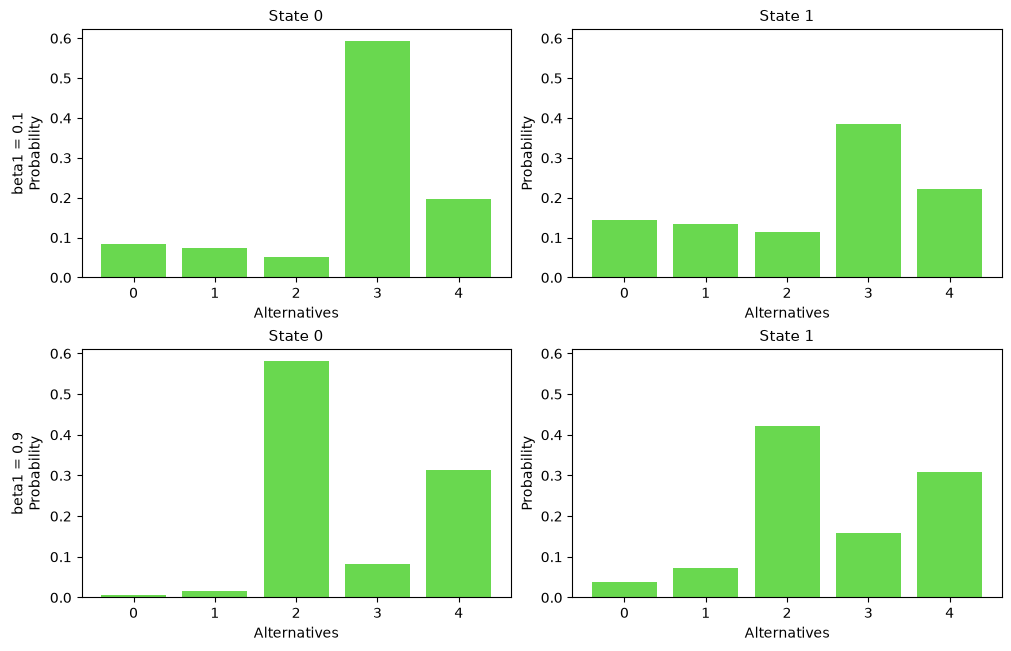
The role of . Same preferences, five times the noise: everything is pulled towards the uniform distribution, exactly as the limit predicts. This is why and the scale of cannot both be identified in the linear model — multiplying and by the same positive constant leaves every choice probability unchanged.
mC = model(nalt=nalt, nattr=nattr, attr=attr, param=mA.param, sigma=5.0, label='sigma = 5')
compare([mA, mC])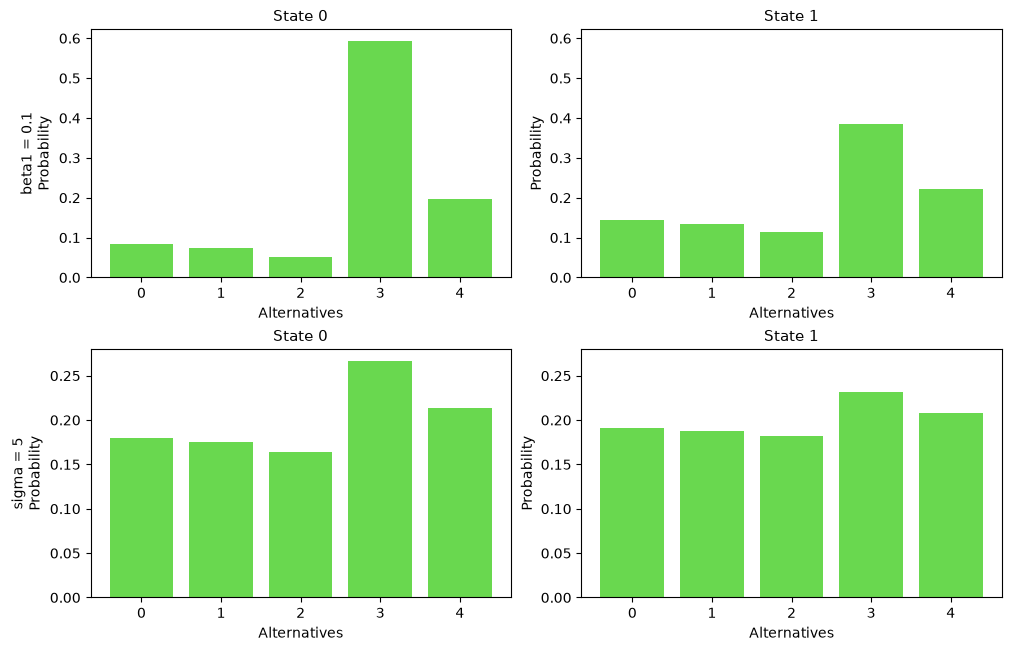
Solution: can all choices concentrate on one alternative?
Yes, and in two different ways — which is the point. Either make one attribute dominate by raising its coefficient, or shrink towards zero so the model approaches deterministic choice. Both produce a degenerate solution, and they are observationally equivalent in the data.
mD = model(nalt=nalt, nattr=nattr, attr=attr, param=np.array([5.1, 0.35, 0.2]), label='large beta1')
mE = model(nalt=nalt, nattr=nattr, attr=attr, param=mA.param, sigma=1e-3, label='tiny sigma')
compare([mD, mE])
Note that mE is only computable because logit de-maxes: with the naive formula
returns nan, as we saw above.
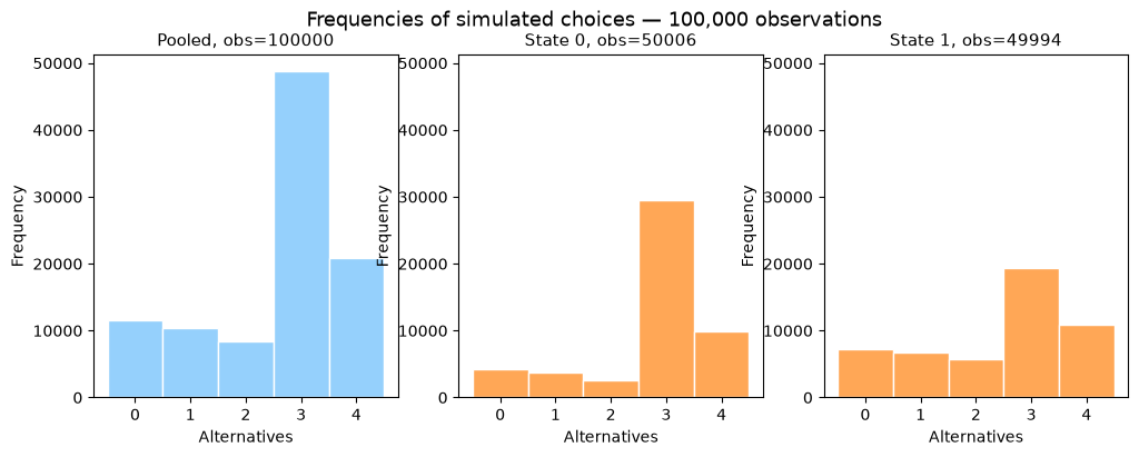
Predicted versus simulated behavior. The solution is a probability; the data is a finite sample from it. With 100 agents the histogram is a rough sketch of the CCPs, with 100,000 it is the CCPs. Estimation is this relation run backwards, and the sampling noise you see here is what standard errors measure.
Source
model_solve(mA)
small = model_simulate(mA, nobs=100, rng=rng)
large = model_simulate(mA, nobs=100_000, rng=rng)
for d, ttl in [(small, '100 observations'), (large, '100,000 observations')]:
    mA.label = ttl
    plot_data(mA, data=d)
    plt.show()
mA.label = 'beta1 = 0.1'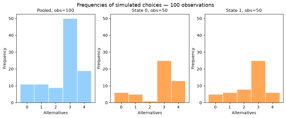
Linear versus log utility. The same means something entirely different once the attributes are logged: differences between alternatives are compressed, so the choice probabilities are flatter, and is no longer a pure normalization.
mF = model(nalt=nalt, nattr=nattr, attr=attr, param=mA.param, util_type='log', label='log utility')
compare([mA, mF])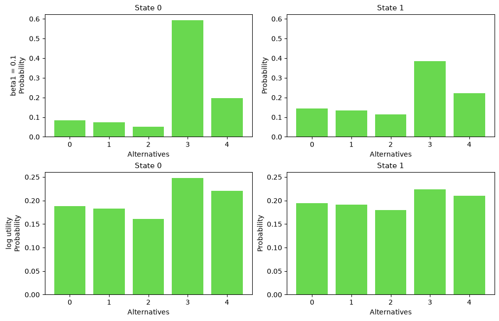
- Thurstone, L. L. (1959). The measurement of values. Univer. Chicago Press.
- Luce, R. D. (1959). Individual choice behavior. John Wiley.
- Marschak, J. (1960). Binary Choice Constraints and Random Utility Indicators. In K. Arrow, S. Karlin, & P. Suppes (Eds.), Mathematical methods in the social sciences, 1959 : proceedings (Vol. viii). Stanford, CA. : Stanford University Press. http://archive.org/details/mathematicalmeth0000stan
- McFadden, D. (1974). Conditional logit analysis of qualitative choice behavior. Frontiers in Econometrics.
- McFadden, D. (1981). Econometric models of probabilistic choice. Structural Analysis of Discrete Data with Econometric Applications, 198272.
- Iskhakov, F., Jørgensen, T., Rust, J., & Schjerning, B. (2017). The endogenous grid method for discrete-continuous dynamic choice models with (or without) taste shocks. Quantitative Economics, 8(2), 317–365. https://doi.org/10.3982/QE643
- Train, K. E. (2009). Discrete Choice Methods with Simulation (2nd ed.). Cambridge University Press. 10.1017/CBO9780511805271