📖 DC-EGM for discrete-continuous choice

🚧 🚧 🚧 Not the final version 🚧 🚧 🚧

The EGM of Class 17 solves the consumption-savings model without a single root-finding operation, but only when the problem is concave. Today we add a discrete choice, retirement, on top of consumption, and code the DC-EGM of Iskhakov et al. (2017): an EGM step per discrete choice, an upper envelope to throw away the points the Euler equation gets wrong, and taste shocks to make the whole thing smooth.

Running the code for this lecture

The code for this class is in the folder session18-oct27/ of the course code repository. We write it together in class, starting from the pre-code notebook dcegm_pre.ipynb, which has the model object and the headings but not the solver. The complete notebook dcegm.ipynb has all the code of this page.

You should have cloned that repository already — if not, the instructions are in the algorithms and complexity lecture.

Update your copy before the class. Editing a file in place makes git pull refuse to update it, so discard whatever you changed while experimenting:

cd sb-dse-code
git reset --hard HEAD
git pull

Nothing in this repository is submitted, so experiment freely — but copy anything you want to keep out of it first, or commit that to a branch of your own.

Setting up the Python environment is covered in Python.

Discrete and continuous choice together¶

In economics the two kinds of choice co-exist:

how much to work, and when to retire or become an entrepreneur
how much to save, and when to buy a house, a car, a durable
which car to buy, and how much to drive it

Traditional methods treat them separately: a discrete choice is a maximum over a finite set, a continuous choice is a first order condition plus concavity, and a dynamic problem is dynamic programming with VFI, policy or time iterations. Put together, the pieces break:

the problem is intrinsically non-concave: the value function is the maximum of several concave functions, one per discrete alternative
first order conditions are not sufficient: the Euler equation has several solutions, and only one is the optimum
value functions have kinks and policy functions have discontinuities, which a fixed grid smears and an optimizer trips over

So a traditional solver needs a global optimizer in every point of the state space, has to locate and track every kink, and needs special numerical procedures for non-smooth objects. DC-EGM keeps the two things EGM is good at, no root finding and an exact treatment of the credit constraint, and adds the machinery for the kinks.

The class of problems is that of EGM, extended:

A1. strictly concave, monotone and differentiable utility
a continuous state $M_t$ , wealth, with the budget constraint as its law of motion
additional discrete states $st_t$ , such as the labor market status, with A2. transition probabilities of $st_t$ independent of $M_t$
one continuous choice $c_t$ , consumption, and one discrete choice $d_t$ , which drives the discrete states

DC-EGM comes in two flavors. Without taste shocks it iterates on the value and policy functions and produces exact thresholds for the discrete decisions. With taste shocks it iterates on choice-specific value functions and produces choice probabilities, as in the Rust model.

Which of the four solvers of Classes 16–17 survives a discrete choice on top of consumption, and at what cost?
Why is the maximum of two concave functions not concave?

The retirement model¶

A worker in state $\mathbb{W}$ chooses consumption $c$ and whether to keep working or retire, $d \in \{\mathbb{W}, \mathbb{R}\}$ . A retiree in state $\mathbb{R}$ only chooses consumption, because retirement is absorbing:

V_t(M_t, \mathbb{W}) = \max\left\{ \begin{array}{l} \max_{0 \leqslant c \leqslant M_t} u(c, \mathbb{R}) + \beta\, \mathbb{E} V_{t+1}\big(\tilde R (M_t - c), \mathbb{R}\big) \\[4pt] \max_{0 \leqslant c \leqslant M_t} u(c, \mathbb{W}) + \beta\, \mathbb{E} V_{t+1}\big(\tilde R (M_t - c) + y, \mathbb{W}\big) \end{array} \right\}

V_t(M_t, \mathbb{R}) = \max_{0 \leqslant c \leqslant M_t} \Big[ u(c, \mathbb{R}) + \beta\, \mathbb{E} V_{t+1}\big(\tilde R (M_t - c), \mathbb{R}\big) \Big]

$\mathbb{R}$ , $\mathbb{W}$ are the retirement and working states $st_t$ , which evolve according to the discrete choices $d \in \{\mathbb{R}, \mathbb{W}\}$
$y$ is the wage, deterministic for now; a retiree has no income
$\tilde R$ is the gross return on savings, possibly random; we keep it fixed at $R$
the horizon is finite, $t = 0, 1, \dots, T-1$ , and in the last period everything is consumed

Utility is additively separable in consumption and the discrete choice, with a disutility of work $\delta$ :

u(c, d) = \frac{c^{\rho} - 1}{\rho} - \delta\, \mathbf{1}(d = \mathbb{W}) \;\;\underset{\rho \to 0}{\longrightarrow}\;\; \log(c) - \delta\, \mathbf{1}(d = \mathbb{W})

The worker’s problem has exactly the EGM structure, choice by choice: fix $d$ , and the post-decision state $A = M - c$ determines next period’s wealth. What is new is the maximum over $d$ in front.

Example: the analytic solution with log utility and no interest

With $u(c) = \log c$ , $R = 1$ and deterministic income the model solves by hand. Let $S_k = \sum_{i=0}^{k} \beta^i$ . A worker with $t$ periods to go consumes a piecewise linear function of wealth:

c^\star(M, \mathbb{W}) = \begin{cases} M & M \leqslant y/\beta \\[2pt] (k y + M) / S_k, \; k = 1, \dots, t-1 & \text{on successive intervals of } M \\[2pt] (k y + M) / S_t, \; k = t, t-1, \dots, 0 & \text{on successive intervals of } M \end{cases}

the first row is the credit constrained consumer, who eats everything and waits for the next paycheck
in the second row the consumer works and smooths consumption over the next $k$ periods, after which the constraint binds again: $k$ grows with wealth
in the third row the constraint never binds, and $k$ is the number of periods the consumer still works before retiring: it falls with wealth, down to $k = 0$ , retirement now

Each row is linear in $M$ , and the rows are stitched together at thresholds $\overline{M}$ that are not in closed form. The slope of the policy and its intercept change at every threshold: those are the kinks and the jumps we are after. The check below compares the numerical solution with this formula.

The analytic consumption rule of a worker, from the DSE 2024 lectures:

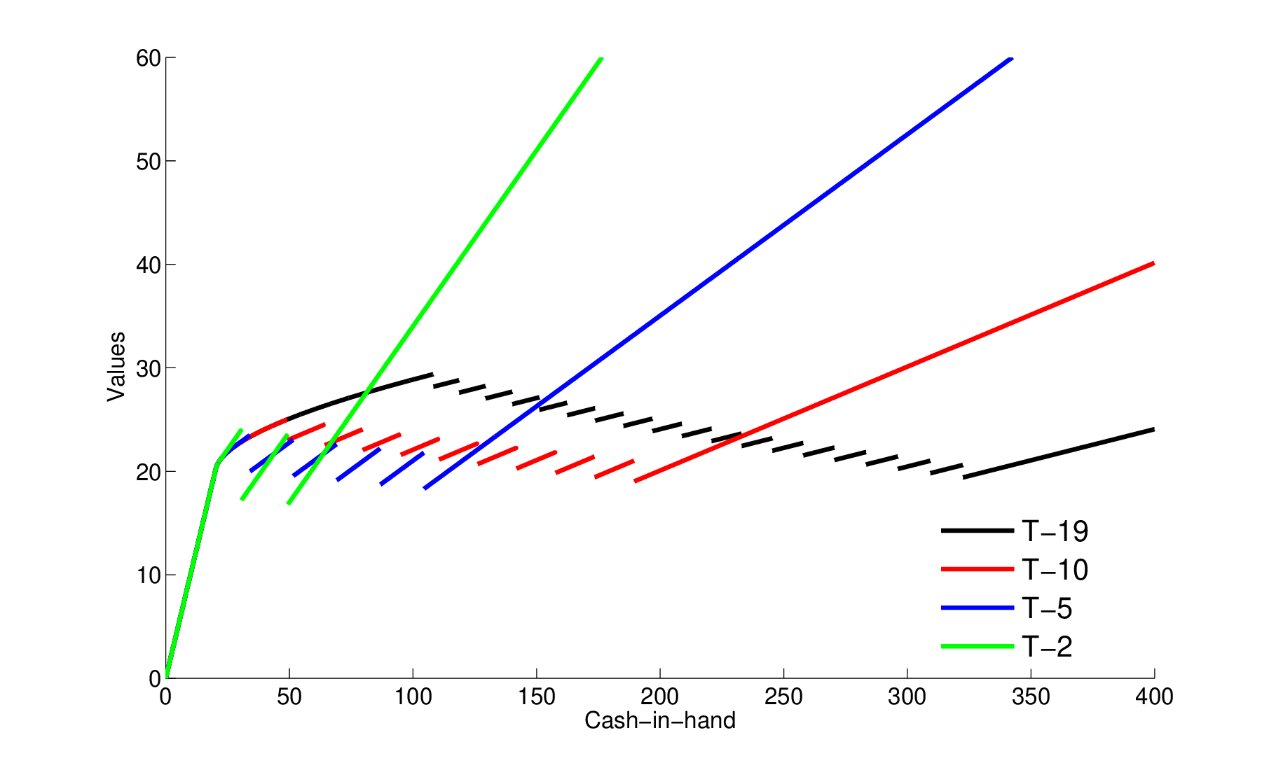
Analytic consumption of a worker at T-2, T-5, T-10 and T-19 against
cash-in-hand M (the vertical axis is consumption), with u(c) = \log c, R = 1,
\beta = 0.98, y = 20 and T = 20. Consumption equals M up to y / \beta, then follows the linear
segments of the formula, and drops at every retirement threshold. — Analytic consumption of a worker at $T-2$ , $T-5$ , $T-10$ and $T-19$ against cash-in-hand $M$ (the vertical axis is consumption), with $u(c) = \log c$ , $R = 1$ , $\beta = 0.98$ , $y = 20$ and $T = 20$ . Consumption equals $M$ up to $y / \beta$ , then follows the linear segments of the formula, and drops at every retirement threshold.

In the analytic solution, why does consumption drop at the thresholds where the consumer decides to retire one period earlier?
What happens to the thresholds as $\beta R$ moves away from one?

The model object follows the architecture of Class 16: parameters, grids, quadrature and the primitives in one place, every solver a function of it. Two details are specific to the discrete choice:

the grid is on savings $A$ , as in EGM, ascending and starting at zero
income is paid only while working, and a retiree with no wealth is kept alive by a consumption floor $\underline{c}$ , the safety net of Iskhakov et al. (2017), which also keeps $\log(0)$ out of the code

import time
import numpy as np
import matplotlib.pyplot as plt
from scipy.optimize import brentq

class retirement():
    '''Consumption-savings model with a discrete retirement choice (Iskhakov et al. 2017)'''

    def __init__(self, beta=0.95, R=1.05, y=1.0, delta=0.5, T=10, sigma=0.0, sigma_y=0.0,
                 Mbar=20, ngrid=500, nquad=5, cfloor=1e-3):
        self.beta, self.R, self.y, self.delta = beta, R, y, delta   # discount, return, wage, disutility of work
        self.T, self.sigma, self.sigma_y = T, sigma, sigma_y  # periods, taste shock scale, income shock std
        self.Mbar, self.ngrid, self.nquad = Mbar, ngrid, nquad
        self.cfloor = cfloor                                  # consumption floor: safety net for a retiree
        self.eps = np.finfo(float).eps                        # smallest positive float
        self.A = np.linspace(0, Mbar, ngrid)                  # grid on savings, ascending, starts at zero
        x, w = np.polynomial.hermite.hermgauss(nquad)         # Gauss-Hermite nodes and weights
        self.quadp = y * np.exp(np.sqrt(2) * sigma_y * x - sigma_y**2 / 2)   # income nodes, mean y
        self.quadw = w / np.sqrt(np.pi)                       # weights, sum to one

    def u(self, c, d):
        return np.log(c) - self.delta * d                     # utility, d = 1 working, d = 0 retired

    def mu(self, c):
        return 1 / c                                          # marginal utility

    def imu(self, x):
        return 1 / x                                          # inverse marginal utility

    def next_wealth(self, A, d, y):
        return np.maximum(self.R * A + d * y, self.cfloor)    # budget: income only while working, safety net

def interp(x, xp, fp):
    '''Linear interpolation, extrapolated linearly beyond the last grid point'''
    slope = (fp[-1] - fp[-2]) / (xp[-1] - xp[-2])
    return np.where(x > xp[-1], fp[-1] + slope * (x - xp[-1]), np.interp(x, xp, fp))

The defaults used in all the figures below, unless stated otherwise:


discount factor, gross return	$\beta = 0.95$ , $R = 1.05$
wage, disutility of work	$y = 1$ , $\delta = 0.5$
utility	$\log c$ , the limit $\rho \to 0$
horizon	$T = 10$ periods, $t = 0, \dots, 9$
savings grid	500 equally spaced points on $[0, 20]$
income shocks	none, $\sigma_y = 0$ ; log-normal with 5 Gauss–Hermite nodes otherwise
taste shocks	none, $\sigma = 0$
consumption floor	$\underline{c} = 10^{-3}$

Periods are indexed from zero, as Python does, so the last period is $T - 1$ and the period before it $T - 2$ .

Choice-specific value functions¶

The plan of Iskhakov et al. (2017) in its first version:

an EGM step for each discrete choice $d$ and every discrete state $st$
this gives the $d$ -specific consumption rules and value functions
compare the $d$ -specific value functions to find the optimal switching points, that is compute their upper envelope
reconstruct the overall consumption rule and value function from the switching points

Nothing here needs a root finder, and the credit constraint keeps its EGM treatment. The price is that we must now compute value functions, which time iterations and EGM never needed, and compute an upper envelope.

So each EGM step must return, for its discrete choice $d$ , the endogenous points $(M_j, c_j)$ and the value at those points,

v_t(M_j, d) = u(c_j, d) + \beta\, \mathbb{E} V_{t+1}\big(R A_j + y\,\mathbf{1}(d = \mathbb{W})\big),

where $V_{t+1}$ is the value of the state the choice $d$ leads to.

The credit constrained region¶

Credit constraints are handled so well by EGM because it never has to evaluate the utility of nearly zero consumption. Instead it “connects the dots” $(0, 0)$ and $(M^{cc}_t, M^{cc}_t)$ , where $M^{cc}_t$ is the wealth level that corresponds to zero savings, $A_t = 0$ : for every $M < M^{cc}_{t}$ the optimal consumption is $c^\star_t = M$ .

Once value functions are needed, the constrained region needs its own formula:

for each $d_t$ the EGM loop starts from $A = 0$ and returns $M^{cc}_{t, d_t}$
for $M < M^{cc}_{t, d_t}$ the value function has the analytic form $V_t^{d_t}(M) = u(M, d_t) + \beta\, EV^{0}_{t+1}(d_t)$ , where $EV^{0}_{t+1}(d_t)$ is the expected value of ending period $t$ with $A_t = 0$ , a number the EGM step computes anyway
with additively separable utility (AS), $V_t^{d_t}(M) = u(M) + v(d_t) + \beta\, EV^0_{t+1}(d_t)$ : the choice-specific value functions differ by a constant for $M < \min_{d_t} M^{cc}_{t, d_t}$ , so they do not intersect there, no switching point has to be searched for at nearly zero wealth, and the choice probabilities do not change

The solution of one period and one choice is therefore a set of endogenous points plus one number, $EV^0$ . The two functions below evaluate the policy and the value anywhere: connecting the dots below the first endogenous point, interpolating above it.

def terminal(m, d):
    '''Last period: everything is consumed, no endogenous points, the whole grid is the constrained region'''
    return {'M': np.array([]), 'c': np.array([]), 'v': np.array([]), 'ev0': 0.0}

def policy(m, s, M):
    '''Consumption at wealth M from the solution s of one period and choice: c = M below the first endogenous point'''
    M = np.asarray(M, float)
    if s['M'].size == 0: return M                             # last period: consume everything
    return np.where(M < s['M'][0], M, interp(M, s['M'], s['c']))

def value(m, s, d, M):
    '''Choice-specific value at wealth M: analytic below the first endogenous point, interpolated above'''
    M = np.asarray(M, float)
    vcc = m.u(np.maximum(M, m.eps), d) + m.beta * s['ev0']    # constrained region: c = M, A = 0
    if s['M'].size == 0: return vcc
    return np.where(M < s['M'][0], vcc, interp(M, s['M'], s['v']))

The discrete choice¶

Next period’s worker chooses again, so the EGM step for $d = \mathbb{W}$ needs the maximum of next period’s two choice-specific values, and the policy of whichever choice wins. The two functions below return that maximum and the indicator of working.

They are written with a scale $\sigma$ of taste shocks already, the subject of the second half of the class: for $\sigma = 0$ they are the plain maximum and the plain indicator.

def logsum(m, vW, vR):
    '''Expected value over the taste shocks: the maximum without shocks, the smoothed logsum with'''
    mx = np.maximum(vW, vR)
    if m.sigma == 0: return mx
    return mx + m.sigma * np.log(np.exp((vW - mx) / m.sigma) + np.exp((vR - mx) / m.sigma))   # de-maxed

def choice_prob(m, vW, vR):
    '''Probability to keep working: an indicator without taste shocks, logit with'''
    if m.sigma == 0: return (vW > vR).astype(float)
    eW, eR = np.exp((vW - np.maximum(vW, vR)) / m.sigma), np.exp((vR - np.maximum(vW, vR)) / m.sigma)
    return eW / (eW + eR)                                     # de-maxed, as in Class 6

The EGM step for one discrete choice¶

The step is the EGM step of Class 17 with two additions: the next period consumption and value depend on which choice is optimal there, and the value at the endogenous points is computed alongside the policy.

Algorithm (EGM step for a discrete choice)

Input: a grid $0 = A_1 < \dots < A_n$ on savings, quadrature nodes and weights $(y_k, \omega_k)$ , the choice $d$ , and next period’s solution for both choices, $\big(c_{t+1}(\cdot, d'), v_{t+1}(\cdot, d')\big)$ , $d' \in \{\mathbb{R}, \mathbb{W}\}$ .

Steps, for every grid point $A_j$ and every node $k$ :

next period wealth: $M'_{jk} = R A_j + y_k\, \mathbf{1}(d = \mathbb{W})$
next period values $v_{t+1}(M'_{jk}, d')$ and consumptions $c_{t+1}(M'_{jk}, d')$ of both choices, and the choice that wins, $P_{jk} = \mathbf{1}\big(v_{t+1}(M'_{jk}, \mathbb{W}) > v_{t+1}(M'_{jk}, \mathbb{R})\big)$ ; if $d = \mathbb{R}$ next period is a retiree and $P_{jk} = 0$
expected marginal utility and expected value over the choice: $\mu_{jk} = P_{jk}\, u'\big(c_{t+1}(M'_{jk}, \mathbb{W})\big) + (1 - P_{jk})\, u'\big(c_{t+1}(M'_{jk}, \mathbb{R})\big)$ , $V'_{jk} = \max_{d'} v_{t+1}(M'_{jk}, d')$
quadrature: $\mathbb{E}\mu_j = \sum_k \omega_k \mu_{jk}$ , $\mathbb{E}V_j = \sum_k \omega_k V'_{jk}$
the inverted Euler equation: $c_j = (u')^{-1}(\beta R\, \mathbb{E}\mu_j)$
the endogenous grid point and the value there: $M_j = A_j + c_j$ , $v_j = u(c_j, d) + \beta\, \mathbb{E}V_j$

Output: the points $(M_j, c_j, v_j)$ , $j = 1, \dots, n$ , and $EV^0 = \mathbb{E}V_1$ , the expected value of saving nothing.

def egm_step(m, d, sol1):
    '''EGM step for choice d (1 work, 0 retire) given the solution sol1 = [retire, work] of next period'''
    M1 = m.next_wealth(m.A[:, None], d, m.quadp[None, :])     # next period wealth: savings x income nodes
    vR = value(m, sol1[0], 0, M1)                             # next period value of a retiree
    cR = np.maximum(policy(m, sol1[0], M1), m.cfloor)         # next period consumption of a retiree
    if d == 1:                                                # still a worker tomorrow: chooses again
        vW = value(m, sol1[1], 1, M1)
        cW = np.maximum(policy(m, sol1[1], M1), m.cfloor)
        P = choice_prob(m, vW, vR)                            # probability to keep working tomorrow
        mu1 = P * m.mu(cW) + (1 - P) * m.mu(cR)               # expected marginal utility over the choice
        V1 = logsum(m, vW, vR)                                # value before the taste shocks are drawn
    else:                                                     # retired tomorrow: no choice
        mu1, V1 = m.mu(cR), vR
    rhs = m.beta * m.R * (mu1 @ m.quadw)                      # RHS of the Euler equation, by quadrature
    c = m.imu(rhs)                                            # inverted Euler equation
    M = m.A + c                                               # endogenous grid points
    ev = V1 @ m.quadw                                         # expected value of next period at each A
    v = m.u(c, d) + m.beta * ev                               # choice-specific value at the endogenous points
    return M, c, v, ev[0]                                     # ev[0]: expected value of saving nothing

Two EGM steps from the terminal period give the last two periods. In the last period a worker never works: there is no future income to earn, so retiring is better by exactly $\delta$ at every wealth level. One period earlier the two choice-specific value functions intersect.

m = retirement()
sol = [[terminal(m, d) for d in (0, 1)]]                      # last period, index T-1
for t in range(2):
    sol.insert(0, [dict(zip(('M', 'c', 'v', 'ev0'), egm_step(m, d, sol[0]))) for d in (0, 1)])   # T-2, then T-3
Mg = np.linspace(0.05, m.Mbar, 1000)                          # dense grid for the plots
fig, ax = plt.subplots(1, 2, figsize=(12, 4.5))
for s, lab in ((sol[2], 'last period'), (sol[1], 'one before last')):
    for d, name in ((0, 'retire'), (1, 'work')):
        ax[0].plot(Mg, value(m, s[d], d, Mg), label=f'{lab}, {name}')
vW, vR = value(m, sol[1][1], 1, Mg), value(m, sol[1][0], 0, Mg)
c = np.where(vW > vR, policy(m, sol[1][1], Mg), policy(m, sol[1][0], Mg))   # the worker's consumption
ax[1].plot(Mg, c, label='worker: retire or work')
ax[1].plot(Mg, policy(m, sol[1][0], Mg), label='retiree')
ax[0].set(ylim=(-3, 5), xlabel='wealth M', title='Choice-specific value functions of a worker')
ax[1].set(ylim=(0, 10.5), xlabel='wealth M', title='Consumption one period before the last')
for a in ax: a.grid(color='0.9'); a.legend()
plt.show()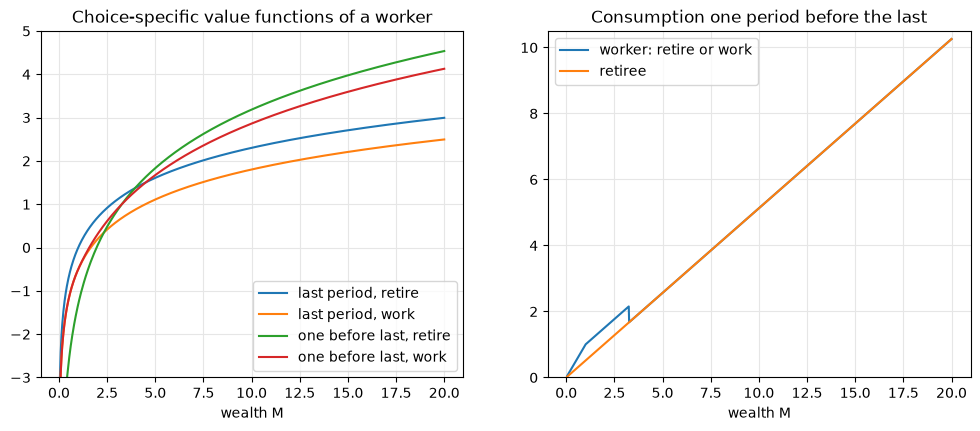

So, what is going on?

the $d$ -specific value functions intersect, due to the trade-off between the income from work and its disutility: a poor worker works, a rich one retires
the upper envelope of the value functions has a kink at the intersection, and the combined consumption function has a discontinuity there: the retiree has no income to look forward to and consumes less out of the same wealth

The kink is the primary kink, the one that comes from the discrete choice itself. The first version of the algorithm handles it: compute both choice-specific functions, find the intersection, and switch.

Why is the consumption of a worker who keeps working higher than that of a retiree at the same wealth, when the worker also pays the disutility $\delta$ ?
The worker’s value function is the maximum of two concave functions. Where is it not concave?

Why the Euler equation is not enough¶

One more period back the trouble starts. The worker’s EGM step now integrates over $V_{T-2}(\cdot, \mathbb{W})$ , which has a kink, so:

the derivative of the value function has a discontinuity at the kink, and so does next period’s consumption, which enters the Euler equation
for some values of wealth the Euler equation has two solutions: one with savings that land below the kink next period, one above
the EGM step, which inverts the Euler equation at every point of the savings grid, returns all of them: the endogenous grid points sorted by savings are no longer sorted by wealth, they bend back and form a zig-zag region

The Euler equation remains a necessary condition for the optimal consumption, as shown by Clausen & Strub (2020) for exactly this kind of non-smooth problem, so the optimum is among the EGM points. It is no longer sufficient: some of the points are not the optimum.

The figure shows the raw output of the worker’s EGM step two periods before the last, zoomed in on the zig-zag, with the points connected in the order of the savings grid. The right panel plots the Euler residual as a function of consumption at a few wealth levels in the region, with the overall consumption rule of next period on the right-hand side.

def euler_residual(m, sol1, M, c):
    '''Euler residual of a worker who keeps working, at wealth M and consumption c, given next period solution'''
    M1 = m.next_wealth(np.asarray(M)[..., None] - np.asarray(c)[..., None], 1, m.quadp)   # ... x nodes
    vW, vR = value(m, sol1[1], 1, M1), value(m, sol1[0], 0, M1)
    P = choice_prob(m, vW, vR)                                # who works next period
    cW, cR = np.maximum(policy(m, sol1[1], M1), m.cfloor), np.maximum(policy(m, sol1[0], M1), m.cfloor)
    return m.mu(c) - m.beta * m.R * ((P * m.mu(cW) + (1 - P) * m.mu(cR)) @ m.quadw)

M, c, v, ev0 = egm_step(m, 1, sol[1])                         # raw EGM step of the worker, two periods before last
bend = np.flatnonzero(np.diff(M) <= 0)                        # steps where the endogenous grid bends back
lo, hi = M[bend].min() - 0.3, M[bend].max() + 0.3             # window around the zig-zag
fig, ax = plt.subplots(1, 3, figsize=(16, 4.5))
ax[0].plot(M, v, '.-', ms=4, lw=0.7)
ax[1].plot(M, c, '.-', ms=4, lw=0.7)
ax[0].set(xlim=(lo, hi), ylim=(np.interp(lo, M, v) - 0.03, np.interp(hi, M, v) + 0.03),
          xlabel='wealth M', title='Value at the EGM points, in savings order')
ax[1].set(xlim=(lo, hi), ylim=(np.interp(lo, M, c) - 0.3, np.interp(hi, M, c) + 0.3),
          xlabel='wealth M', title='Consumption at the EGM points')
cg = np.linspace(1.6, 2.6, 500)
for Mz in np.linspace(lo + 0.1, hi - 0.1, 5):
    ax[2].plot(cg, euler_residual(m, sol[1], Mz, cg), lw=0.8, label=f'M = {Mz:.2f}')
ax[2].axhline(0, color='k', lw=0.5)
ax[2].set(ylim=(-0.15, 0.15), xlabel='consumption c', title='Euler residuals: several zeros'); ax[2].legend()
for a in ax: a.grid(color='0.9')
plt.show()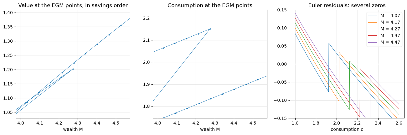

What the figure shows:

the curve of endogenous points goes up, turns back, and goes up again: three monotone segments, of which the middle one and parts of the other two are suboptimal
in consumption, the same wealth level has two candidate values, roughly 0.15 apart
the Euler residual crosses zero twice for every wealth level in the window

The EGM step has no way of telling which crossing is the optimum: that needs the value at the two points.

Time iterations solve the Euler equation in every state with a root finder. Which of the two zeros would brentq return?
The kink of $V_{T-2}(\cdot, \mathbb{W})$ sits at one wealth level. Why does the zig-zag in period $T-3$ spread over an interval of wealth?

The secondary upper envelope¶

How to detect the zig-zag regions algorithmically? The theorem from Class 17 still holds:

Note that the savings function may still have upward jumps. The theorem turns the detection into a sorting problem:

sort the exogenous grid over $A$ in ascending order
then the sequence of endogenous grid points over $M$ has to be in ascending order as well, as long as the Euler equation is sufficient
every time the endogenous grid bends back, it is separated into subsets of points
calculate the upper envelope of the value function over the segments
delete the suboptimal endogenous points
find and add the kink point to the endogenous grid

The kink point is where two segments of the value function cross. Consumption is discontinuous there, so it enters the policy twice: with the consumption of the left segment and with the consumption of the right one. This is the secondary kink, which comes from the primary kink of the next period propagated through the Euler equation.

Algorithm (upper envelope of the endogenous points)

Input: the endogenous points $(M_j, c_j, v_j)$ , $j = 1, \dots, n$ , in the order of the savings grid, the choice $d$ and $EV^0$ .

Steps:

Split the index sequence $1, \dots, n$ into maximal runs on which $M_j$ is monotone, sharing the turning points; flip the descending runs. If there is one run, stop.
Add the credit constrained segment, the analytic value $u(M, d) + \beta EV^0$ with $c = M$ , as one more line; it is only needed at wealth points below $M_1$ .
Collect all wealth values $x_1 < \dots < x_K$ of all runs. For every run $r$ and every $x_k$ inside the run’s interval let $V_{rk}$ be the linear interpolation of the run’s values at $x_k$ ; a run is never evaluated outside its own interval. Let $\tau_k = \arg\max_r V_{rk}$ be the run on top at $x_k$ .
Keep the original point $j$ if $v_j = \max_r V_{rk}$ at $x_k = M_j$ ; delete it otherwise.
For every $k$ with $\tau_k \neq \tau_{k+1}$ : no run has a point strictly inside $[x_k, x_{k+1}]$ , so every run that covers it is a straight line there, and two such lines cross in closed form from their values at $x_k$ and $x_{k+1}$ . Starting from $\ell = \tau_k$ at $z = x_k$ , find the line that overtakes $\ell$ first after $z$ , move $z$ to that crossing and $\ell$ to that line, and repeat until $\ell = \tau_{k+1}$ . At every crossing insert two points: one with the consumption of the line on the left, one with that of the line on the right, both with the value at the crossing. If one of the two lines is the constrained segment, which is concave rather than straight, refine the crossing with a root finder on the analytic value.
Sort the surviving and the new points by $M$ .

Output: the cleaned points $(M_j, c_j, v_j)$ , ascending in $M$ .

In code the runs are index arrays. Each run is interpolated only on the wealth points that fall inside its own interval, and the envelope is built by letting the runs overwrite it one at a time where they are higher. The cost is the number of points plus the number of points in the overlapping regions, which is linear in the grid size. A matrix of all runs on all points would cost (runs) × (points), and interpolate every run on hundreds of points where it is not even defined.

def segments(M):
    '''Indices of the maximal monotone runs of M, each run ascending in M, the turning points shared'''
    up = np.diff(M) > 0                                       # direction of every step
    turn = np.flatnonzero(up[1:] != up[:-1]) + 1              # steps where the direction changes
    bounds = np.r_[0, turn, M.size - 1]
    runs = [np.arange(a, b + 1) for a, b in zip(bounds[:-1], bounds[1:])]
    return [r if M[r[-1]] > M[r[0]] else r[::-1] for r in runs]   # flip the descending runs

The lines: the credit constrained curve as line 0, then one line per run, each on the slice of wealth points it covers.

def envelope_lines(m, d, M, c, v, ev0, runs):
    '''Every run on the wealth points inside its own interval, the envelope, and the line on top at every point'''
    x = np.sort(M, kind='stable')                             # all wealth points; a stable sort merges the sorted runs
    x = x[np.r_[True, np.diff(x) > 0]]                        # drop the duplicates: the shared turning points
    ncc = np.searchsorted(x, M[0])                            # points below the first endogenous point, if any
    lines = [(0, ncc, m.u(x[:ncc], d) + m.beta * ev0, x[:ncc])]   # line 0: credit constrained, c = M, analytic value
    for r in runs:
        lo, hi = np.searchsorted(x, M[r[0]]), np.searchsorted(x, M[r[-1]], 'right')   # x-points inside the run
        lines.append((lo, hi, np.interp(x[lo:hi], M[r], v[r]), np.interp(x[lo:hi], M[r], c[r])))
    vmax, top = np.full(x.size, -np.inf), np.full(x.size, -1) # the envelope and the line on top at every point
    for i, (lo, hi, V, C) in enumerate(lines):
        better = V > vmax[lo:hi]                              # where this line beats the envelope so far
        vmax[lo:hi] = np.where(better, V, vmax[lo:hi])
        top[lo:hi] = np.where(better, i, top[lo:hi])
    return x, lines, vmax, top

The kink: two straight lines on one interval cross in closed form; only the constrained curve, which is concave, needs the root finder.

def crossing(m, d, ev0, x, lines, a, b, j):
    '''Kink where line b overtakes line a on [x[j], x[j+1]]: wealth, value, consumption left and right'''
    (lo0, hi0, V0, C0), (lo1, hi1, V1, C1) = lines[a], lines[b]
    if not (lo0 <= j < hi0 - 1 and lo1 <= j < hi1 - 1): return None   # a line ends or starts here: no crossing
    f0, f1 = V1[j - lo1] - V0[j - lo0], V1[j + 1 - lo1] - V0[j + 1 - lo0]   # difference of the lines at both ends
    if f0 * f1 >= 0: return None                              # no sign change: the lines share the point
    at = lambda A, lo, w: A[j - lo] + w * (A[j + 1 - lo] - A[j - lo])   # a line evaluated at x[j] + w (x[j+1] - x[j])
    w = f0 / (f0 - f1)                                        # both lines straight on [x[j], x[j+1]]: closed form
    z, vz = x[j] + w * (x[j + 1] - x[j]), at(V0, lo0, w)       # the kink and the value there
    if a == 0 or b == 0:                                      # the constrained curve is concave: refine by a root finder
        lo, V = (lo1, V1) if a == 0 else (lo0, V0)            # the run that crosses it
        g = lambda z: m.u(z, d) + m.beta * ev0 - at(V, lo, (z - x[j]) / (x[j + 1] - x[j]))
        z = brentq(g, x[j], x[j + 1])
        w, vz = (z - x[j]) / (x[j + 1] - x[j]), m.u(z, d) + m.beta * ev0
    return z, vz, at(C0, lo0, w), at(C1, lo1, w)              # consumption jumps at the kink: left line, right line

The envelope itself: keep the original points that sit on top, add the kinks, sort. Usually the line on top at $x_{k+1}$ overtakes the one on top at $x_k$ directly, but a third line can sit above both in the middle of the interval, so the code walks through the crossings one at a time.

def upper_envelope(m, d, M, c, v, ev0):
    '''Delete the endogenous points below the upper envelope of the curve (M, v), insert the kinks'''
    runs = segments(M)
    if len(runs) == 1: return M, c, v                         # no bend-back: nothing to do
    x, lines, vmax, top = envelope_lines(m, d, M, c, v, ev0, runs)
    vM = vmax[np.searchsorted(x, M)]                          # the envelope at the original points
    keep = v >= vM - 1e-10 * (1 + np.abs(vM))                 # keep the points on the envelope only
    Mn, cn, vn = [M[keep]], [c[keep]], [v[keep]]
    for j in np.flatnonzero(np.diff(top)):                    # the top line changes between x[j] and x[j+1]
        a, z = top[j], x[j]                                   # walk from the line on top at x[j] ...
        while a != top[j + 1]:                                # ... to the line on top at x[j+1]
            first = None                                      # the first line to overtake a after z
            for b in range(len(lines)):
                k = None if b == a else crossing(m, d, ev0, x, lines, a, b, j)
                if k is not None and k[0] > z and (first is None or k[0] < first[0][0]): first = (k, b)
            if first is None: break                           # the lines only share a point here
            (z, vz, c0, c1), a = first
            Mn.append([z - 1e3 * m.eps, z]); vn.append([vz, vz]); cn.append([c0, c1])   # the kink, twice
    Mn, cn, vn = map(np.concatenate, (Mn, cn, vn))
    i = np.argsort(Mn, kind='stable')                         # nearly sorted already: linear time
    return Mn[i], cn[i], vn[i]

The tolerance in the keep line matters: a point of a suboptimal segment can sit 10^-5 below the envelope, and np.isclose with its default tolerance would keep it, a stray point that puts a spurious jump into the policy. Linear interpolation reproduces a point’s own value to machine precision, so the tolerance can be tight. The crossing is computed from the values of the two lines at the ends of one interval, so it costs nothing beyond the interpolation already done.

Mc, cc, vc = upper_envelope(m, 1, M, c, v, ev0)             # the raw points of the figure above, cleaned
fig, ax = plt.subplots(1, 2, figsize=(12, 4.5))
ax[0].plot(M, v, '.-', ms=4, lw=0.7, color='0.6', label='EGM points, in savings order')
ax[0].plot(Mc, vc, 'o-', ms=3, lw=1, color='C3', label='after the upper envelope')
ax[1].plot(M, c, '.-', ms=4, lw=0.7, color='0.6', label='EGM points, in savings order')
ax[1].plot(Mc, cc, 'o-', ms=3, lw=1, color='C3', label='after the upper envelope')
ax[0].set(xlim=(lo, hi), ylim=(np.interp(lo, M, v) - 0.03, np.interp(hi, M, v) + 0.03),
          xlabel='wealth M', title='Value: the upper envelope and the secondary kink')
ax[1].set(xlim=(lo, hi), ylim=(np.interp(lo, M, c) - 0.3, np.interp(hi, M, c) + 0.3),
          xlabel='wealth M', title='Consumption: the jump at the secondary kink')
for a in ax: a.grid(color='0.9'); a.legend()
print(f'{M.size} endogenous points in, {Mc.size} out: {np.sum(~np.isin(Mc, M))} inserted at the kink')
plt.show()

500 endogenous points in, 494 out: 2 inserted at the kink

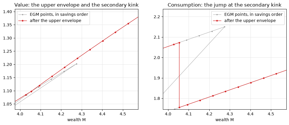
The middle segment and the tails of the other two are gone, the value function has a kink where the two surviving segments cross, and consumption jumps down at that point: the consumer who saves a little more lands above next period’s retirement threshold, and behaves differently from there on.

Where it breaks:

a zig-zag region narrower than the grid spacing is missed: no bend-back, no envelope, and the kink is smeared between two grid points as on a fixed grid
when the discrete choices are very different the $d$ -specific endogenous grids may not overlap, and the comparison of the value functions needs extrapolation

An alternative that does not rely on the monotonicity of savings is the fast upper-envelope scan of Dobrescu & Shanker (2022):

sort the endogenous points by wealth, and choose a jump threshold for consumption
walking along the sorted points, delete a point as inferior whenever the value decreases while consumption jumps at the same time

It generalizes to higher dimensions, at the price of a pre-set threshold that can mis-classify points. FUES is the default secondary envelope of the dcegm package of Maximilian Blesch and coauthors (see the references), with the fixed-grid envelope of Druedahl & Jørgensen (2017) as the alternative; the implementation above is the original DC-EGM envelope of Iskhakov et al. (2017), made local.

Which runs can be on top in step 3 of the algorithm, and why is the credit constrained segment included at all?
Count the operations of envelope_lines as a function of the number of points $n$ and the number of runs. Which part is intrinsic to the problem, and which would a matrix of all runs on all points add?
The kink point is inserted twice in the policy, 10^-13 apart. What would a single point do to the linear interpolation of consumption?

The full algorithm without taste shocks¶

Algorithm (DC-EGM, backward induction)

Input: the grids, nodes and weights of the model, and the horizon $T$ .

Iterate backward for $t = T-2, T-3, \dots, 0$ , starting from the terminal solution $c_{T-1}(M, d) = M$ , $v_{T-1}(M, d) = u(M, d)$ :

for each discrete choice $d \in \{\mathbb{R}, \mathbb{W}\}$ : take the EGM step with next period’s solution, to obtain the $d$ -specific consumption rule and value function on the endogenous grid
for the worker’s choice $d = \mathbb{W}$ : compute the secondary upper envelope over the zig-zag regions of the $d$ -specific value function, and update the corresponding consumption rule
compare the $d$ -specific value functions to find the optimal switching points, the primary upper envelope
reconstruct the overall consumption rule and value function of the worker from the switching points

Output: $c_t(M, d)$ and $v_t(M, d)$ for all $t$ and $d$ , from which the worker’s policy is $d_t(M) = \arg\max_d v_t(M, d)$ and $c_t(M) = c_t(M, d_t(M))$ .

Steps 1 and 2 are the solver. Steps 3 and 4 are done on demand, by comparing the two interpolated value functions at any wealth level: the function worker below is the primary envelope. The retiree’s curve never bends back, because the retiree’s problem is concave, so only the worker’s step runs the envelope.

def solve_dcegm(m, callback=None):
    '''Backward induction with DC-EGM: returns sol[t][d], t = 0..T-1, d = 0 retire, 1 work'''
    sol = [[None, None] for t in range(m.T)]
    sol[-1] = [terminal(m, d) for d in (0, 1)]
    for t in range(m.T - 2, -1, -1):
        for d in (0, 1):
            M, c, v, ev0 = egm_step(m, d, sol[t + 1])
            if d == 1:                                        # only the worker's curve can bend back
                M, c, v = upper_envelope(m, d, M, c, v, ev0)
            sol[t][d] = {'M': M, 'c': c, 'v': v, 'ev0': ev0}
            assert np.all(np.diff(M) > 0)                     # the cleaned endogenous grid is sorted
            if callback: callback(t=t, d=d, sol=sol[t][d])
    return sol

def worker(m, sol_t, M):
    '''Policy of a worker in one period: consumption, the probability to work, and the value'''
    vW, vR = value(m, sol_t[1], 1, M), value(m, sol_t[0], 0, M)
    P = choice_prob(m, vW, vR)
    c = np.where(P > 0.5, policy(m, sol_t[1], M), policy(m, sol_t[0], M))   # the more likely choice
    return c, P, logsum(m, vW, vR)

t0 = time.perf_counter()
sol = solve_dcegm(m)
print(f'DC-EGM solved {m.T} periods on {m.ngrid} grid points in {time.perf_counter() - t0:.3f} seconds')
fig, ax = plt.subplots(1, 3, figsize=(16, 4.5))
for t, col in zip(range(m.T - 1), plt.cm.viridis(np.linspace(0, 0.9, m.T - 1))):
    c, P, V = worker(m, sol[t], Mg)
    ax[0].plot(Mg, c, color=col, lw=0.9, label=f't = {t}')
    ax[1].plot(Mg, V, color=col, lw=0.9)
    ax[2].plot(Mg, P, color=col, lw=0.9)
ax[0].set(ylim=(0, 8), xlabel='wealth M', title="Worker's consumption, t = 0 (dark) to T-2 (light)")
ax[1].set(ylim=(-4, 10), xlabel='wealth M', title="Worker's value function")
ax[2].set(xlabel='wealth M', title='Decision to keep working')
ax[0].legend(fontsize=8)
for a in ax: a.grid(color='0.9')
plt.show()

DC-EGM solved 10 periods on 500 grid points in 0.013 seconds

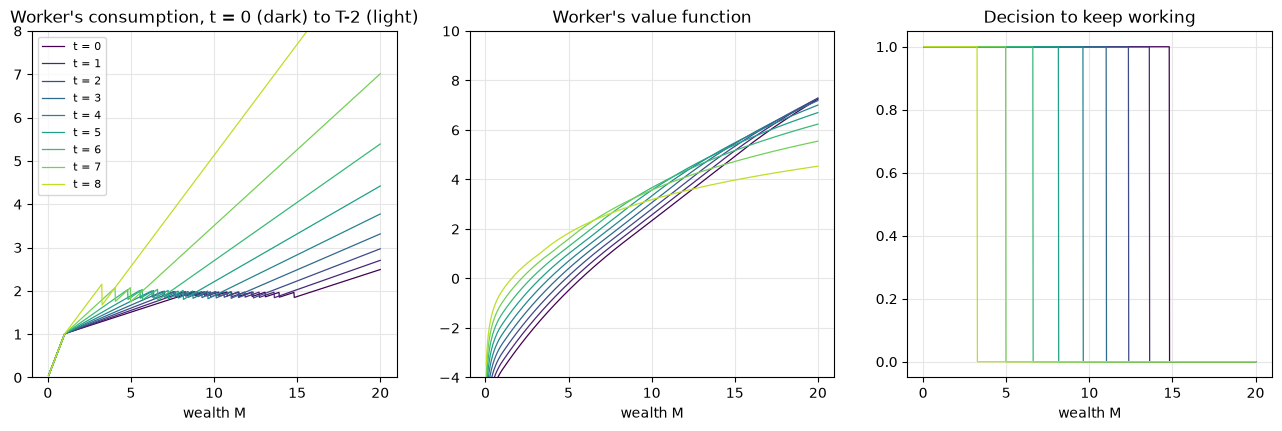
Properties of the full solution, all of them attributes of the model itself and not of the method:

value functions are non-concave and have kinks, one primary kink per period at the retirement threshold, which moves out as the horizon grows
consumption functions have discontinuities: the drop at the retirement threshold and, to the left of it, the smaller drops at the secondary kinks
the discontinuities and kinks propagate through time and accumulate: the policy in period 0 carries the image of every future threshold, a snowball of jumps

Any solution method has to deal with these complexities. A solver on a fixed grid sees them as noise.

Check against the analytic solution¶

With $R = 1$ the analytic policy is a list of candidate lines. The check evaluates the numerical policy on a dense grid and reports the distance to the nearest candidate.

ma = retirement(R=1.0)                                        # log utility, no interest: analytic case
sa = solve_dcegm(ma)
S = lambda k: sum(ma.beta**i for i in range(k + 1))           # S_k = 1 + beta + ... + beta^k
for t in (0, 4, 7, 8):
    tg = ma.T - 1 - t                                         # periods to go
    c, P, V = worker(ma, sa[t], Mg)
    lines = [Mg] + [(k * ma.y + Mg) / S(k) for k in range(1, tg)] + [(k * ma.y + Mg) / S(tg) for k in range(tg + 1)]
    dev = np.min(np.abs(np.array(lines) - c), axis=0)         # distance to the nearest analytic line
    print(f'{tg} periods to go: {np.mean(dev < 1e-10) * 100:5.1f}% of the grid points within 1e-10 of the '
          f'analytic policy, max deviation {dev.max():.1e} at M = {Mg[dev.argmax()]:.2f}')

9 periods to go:  84.5% of the grid points within 1e-10 of the analytic policy, max deviation 2.1e-03 at M = 1.17
5 periods to go:  95.7% of the grid points within 1e-10 of the analytic policy, max deviation 2.1e-03 at M = 1.17
2 periods to go:  99.7% of the grid points within 1e-10 of the analytic policy, max deviation 2.1e-03 at M = 1.17
1 periods to go: 100.0% of the grid points within 1e-10 of the analytic policy, max deviation 1.8e-15 at M = 10.67

DC-EGM matches the analytic solution to machine precision on most of the grid, and on all of it one period before the end: the retirement thresholds and the jumps are placed exactly.

The deviations, at most $2 \cdot 10^{-3}$ and starting at $M \approx 1.15$ , sit at the kinks of the second row of the analytic formula and at their images in earlier periods. A kink that comes from the credit constraint binding two periods ahead is not an endogenous grid point, so linear interpolation smears it like on any fixed grid, and the error spreads the longer the horizon.

The run time is a few milliseconds for ten periods. Which part of the algorithm is not vectorized, and when would it dominate?
Why does the accumulation of kinks make a finer grid more necessary in period 0 than in period $T-2$ ?

Random income¶

Random shocks do help. With a log-normal wage the expectation in the Euler equation averages next period’s consumption rule over the income nodes, and the jump at the retirement threshold is spread over a range of savings. However:

shocks smooth out secondary kinks only: the primary kinks, the switching between the discrete options, remain
they may not smooth out all of them: a continuous but sharp decline in consumption at $t$ can still produce a discontinuity or a kink at $t - 1$
the expectations in the Euler equation are now taken over discontinuous functions, and quadrature assumes a smooth integrand: more kinks appear from sloppy computation, and a careful implementation integrates over the continuous intervals separately

t = m.T - 4
fig, ax = plt.subplots(1, 2, figsize=(12, 4.5))
for sy, nq, ls in ((0, 5, '-'), (0.2, 5, '-'), (0.5, 5, '-'), (0.5, 30, ':')):
    ms = retirement(sigma_y=sy, nquad=nq)
    c, P, V = worker(ms, solve_dcegm(ms)[t], Mg)
    ax[0].plot(Mg, c, ls, lw=1, label=f'σ_y = {sy}, {nq} nodes')
    ax[1].plot(Mg, P, ls, lw=1)
ax[0].set(xlim=(2, 9), ylim=(1.3, 2.6), xlabel='wealth M', title=f'Consumption of a worker, t = {t}')
ax[1].set(xlabel='wealth M', title='Decision to keep working')
ax[0].legend()
for a in ax: a.grid(color='0.9')
plt.show()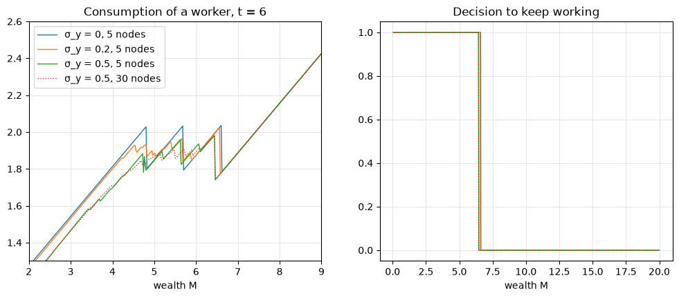

With $\sigma_y = 0.5$ the secondary jumps have become smooth dips, and the primary drop at the retirement threshold is as sharp as before. With 5 quadrature nodes the dips carry small spurious kinks, one per node crossing the threshold: 30 nodes remove them.

Why can an income shock never smooth the primary kink of the same period?
The expectation of a discontinuous function by Gauss–Hermite quadrature is itself a discontinuous function of savings. Where exactly are its jumps?

Extreme value taste shocks¶

Taste shocks smooth out the primary kinks too. Add to each discrete alternative an additive shock $\sigma \epsilon_d$ , i.i.d. extreme value type 1, as in the logit of Class 6:

the extreme value distribution gives closed form expectations, and is standard in empirical applications
two interchangeable interpretations: structural, the shocks are unobserved state variables, or logit smoothing, a device to streamline the solution
they work together with the other shocks of the model: taste shocks smooth the primary kinks, random income or returns smooth the secondary ones
complete smoothing is not guaranteed in general: secondary kinks may persist

Re-formulate the worker’s problem in terms of choice-specific value functions:

V_t(M_t, \mathbb{W}) = \max\left\{ \begin{array}{l} v_t(M_t, \mathbb{W}, \mathbb{R}) + \sigma \epsilon_{\mathbb{R}} \\ v_t(M_t, \mathbb{W}, \mathbb{W}) + \sigma \epsilon_{\mathbb{W}} \end{array} \right\}

\begin{aligned} v_t(M_t, \mathbb{W}, \mathbb{W}) &= \max_{0 \leqslant c \leqslant M_t} \Big[ u(c) + \beta\, EV_{t+1}\big(\tilde R (M_t - c) + y, \mathbb{W}\big) \Big] \\ v_t(M_t, \mathbb{W}, \mathbb{R}) &= \max_{0 \leqslant c \leqslant M_t} \Big[ u(c) + \beta\, EV_{t+1}\big(\tilde R (M_t - c), \mathbb{R}\big) \Big] \end{aligned}

The expected value of a worker, before the shocks are drawn, is the logsum of Class 6:

EV_{t+1}(x, \mathbb{W}) = \sigma \log\Big[ \exp\frac{v_{t+1}(x, \mathbb{W}, \mathbb{W})}{\sigma} + \exp\frac{v_{t+1}(x, \mathbb{W}, \mathbb{R})}{\sigma} \Big]

and the retiree’s problem is unchanged, $V_t(M_t, \mathbb{R}) = \max_{c} [u(c) + \beta EV_{t+1}(\tilde R(M_t - c), \mathbb{R})]$ .

The smoothed Euler equation¶

Without taste shocks the Euler equation is discontinuous in savings, because next period’s consumption is that of either a worker or a retiree:

u'(c_t) = \beta\, \mathbb{E}\Big[ u'\big(c_{t+1}(\mathbb{W}/\mathbb{R})\big)\, \tilde R \Big]

With extreme value taste shocks the Euler equation is smoothed: the marginal utility of next period is averaged over the two choices with the choice probabilities,

u'(c_t) = \beta\, \mathbb{E}\Big[ P_{t+1}(\mathbb{W})\, u'\big(c_{t+1}(\mathbb{W})\big)\, \tilde R + P_{t+1}(\mathbb{R})\, u'\big(c_{t+1}(\mathbb{R})\big)\, \tilde R \Big],

where the probability to keep working is the logit

P_{t+1}(\mathbb{W}) = \frac{\exp\frac{v_{t+1}(M_{t+1}, \mathbb{W}, \mathbb{W})}{\sigma}} {\exp\frac{v_{t+1}(M_{t+1}, \mathbb{W}, \mathbb{W})}{\sigma} + \exp\frac{v_{t+1}(M_{t+1}, \mathbb{W}, \mathbb{R})}{\sigma}}

This is exactly what egm_step computes with choice_prob and logsum when $\sigma > 0$ : the code of the first half of the class was written for both flavors. The de-maxing of Class 6 is essential, because $v/\sigma$ overflows exp for any small $\sigma$ .

Algorithm (DC-EGM with taste shocks)

Input: as before, plus the scale $\sigma > 0$ .

Iterate backward for $t = T-2, \dots, 0$ from the terminal solution:

for each discrete choice $d$ : the EGM step with next period’s choice-specific solution, with the expected marginal utility weighted by the choice probabilities and the expected value given by the logsum
for the worker’s choice: the secondary upper envelope over the zig-zag regions, if any
dropped: compare the $d$ -specific value functions to find the optimal switching points
dropped: reconstruct the overall consumption rule and value function

Output: the choice-specific $c_t(M, d)$ and $v_t(M, d)$ ; the policy is the choice probability $P_t(\mathbb{W} \mid M)$ and the consumption conditional on the choice.

With taste shocks DC-EGM becomes simpler:

the problem is re-formulated in terms of choice-specific value functions
the calculation of the primary upper envelope is replaced by the logsum
expectations are easier to compute, because there are fewer discontinuities
more memory is required, to store the choice-specific value functions

How far is the smoothed solution from the exact one? The paper gives a bound.

This implies that the extreme value perturbed policy functions $c_{\sigma, t}(s, \epsilon)$ and $d_{\sigma, t}(s, \epsilon)$ converge pointwise to $c_t(s)$ and $d_t(s)$ , the optimal continuous and discrete decision rules of the problem without taste shocks, as $\sigma \to 0$ .

This is the extreme value homotopy: solve with a comfortable $\sigma$ , and reduce it towards the sharp problem if needed.

fig, ax = plt.subplots(1, 3, figsize=(16, 4.5))
Mz = 0.5 * (lo + hi)                                          # a wealth level inside the zig-zag region
for s in (0, 0.01, 0.05, 0.1):
    ms = retirement(sigma=s)
    ss = solve_dcegm(ms)
    c, P, V = worker(ms, ss[t], Mg)
    ax[0].plot(Mg, policy(ms, ss[t][1], Mg), lw=1, label=f'σ = {s}')   # consumption conditional on working
    ax[1].plot(Mg, P, lw=1)
    ax[2].plot(cg, euler_residual(ms, ss[m.T - 2], Mz, cg), lw=1)
ax[0].set(xlim=(2, 9), ylim=(1.3, 2.6), xlabel='wealth M', title=f'Consumption of a worker who keeps working, t = {t}')
ax[1].set(xlabel='wealth M', title='Probability to keep working')
ax[2].axhline(0, color='k', lw=0.5)
ax[2].set(ylim=(-0.15, 0.15), xlabel='consumption c', title=f'Euler residual at M = {Mz:.2f}, t = T-3')
ax[0].legend()
for a in ax: a.grid(color='0.9')
plt.show()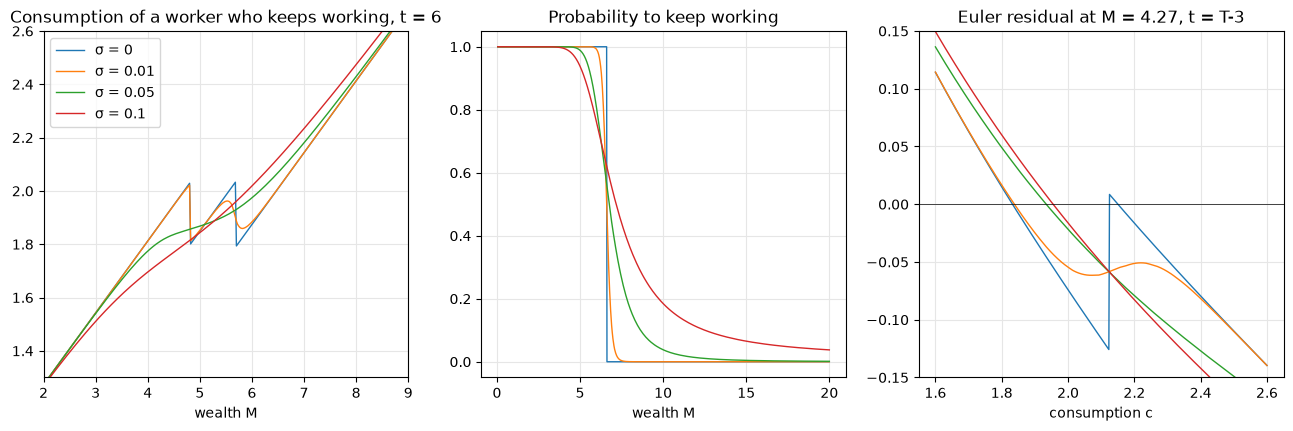

Consumption: the left panel is the choice-specific policy $c_t(M, \mathbb{W})$ , because with taste shocks the overall consumption is a lottery between the two choice-specific ones. Already with $\sigma = 0.01$ the secondary jumps turn into smooth dips, and with $\sigma = 0.1$ the policy is smooth everywhere
Choice probability: the step at the retirement threshold becomes a logit curve, wider the larger $\sigma$ ; with $\sigma = 0.1$ a worker with twice the threshold wealth still works with probability close to 0.1
Euler residual: the two zeros of the discontinuous residual merge into one zero of a continuous function; the zig-zag never forms, and the upper envelope has nothing to do

Where it breaks: $\sigma$ is a structural parameter if the shocks are interpreted as unobserved states, and a numerical one otherwise. A large $\sigma$ changes the economics of the model, a small one brings the kinks back, and the bound of the theorem is the only guide to how far a given $\sigma$ is from the sharp problem.

Taste shocks make the EGM step simpler and the solution better behaved, and the paper still presents the version without them in full. Why?
Which parts of the course notation does $\sigma$ collide with, and which object in the Rust model of Class 9 plays its role?

Simulation¶

The simulator draws the taste shocks through the choice probability and the income shocks from the log-normal, and applies the choice-specific policies. Retirement is absorbing, so the discrete state is carried forward.

def simulate(m, sol, M0, seed=None):
    '''Simulate the life cycle of workers from initial wealth M0 (array): wealth, consumption, work status'''
    rng = np.random.default_rng(seed)
    N = np.atleast_1d(M0).size
    M, C, D = np.empty((N, m.T)), np.empty((N, m.T)), np.ones((N, m.T), int)
    M[:, 0] = M0
    for t in range(m.T):
        if t > 0: D[:, t] = D[:, t - 1]                       # retirement is absorbing
        w = D[:, t] == 1                                      # those still working decide
        vW, vR = value(m, sol[t][1], 1, M[w, t]), value(m, sol[t][0], 0, M[w, t])
        D[w, t] = rng.random(w.sum()) < choice_prob(m, vW, vR)   # taste shocks, through the logit
        for d in (0, 1):
            i = D[:, t] == d
            C[i, t] = policy(m, sol[t][d], M[i, t])           # consumption conditional on the choice
        if t < m.T - 1:
            y = m.y * np.exp(m.sigma_y * rng.standard_normal(N) - m.sigma_y**2 / 2)   # income draws
            M[:, t + 1] = m.next_wealth(M[:, t] - C[:, t], D[:, t], y)
    return M, C, D

ms = retirement(sigma=0.1, sigma_y=0.2, nquad=10)
ss = solve_dcegm(ms)
M0 = np.random.default_rng(1).uniform(2, 20, 1000)            # initial wealth of 1000 workers
Ms, Cs, Ds = simulate(ms, ss, M0, seed=2026)
age = np.where((Ds == 0).any(axis=1), np.argmin(Ds, axis=1), ms.T)   # first period of retirement
fig, ax = plt.subplots(1, 3, figsize=(16, 4.5))
for i in range(15):
    ax[0].plot(Ms[i], lw=0.8, color='C0'); ax[1].plot(Cs[i], lw=0.8, color='C1')
    if age[i] < ms.T:
        ax[0].plot(age[i], Ms[i, age[i]], 'ks', ms=4); ax[1].plot(age[i], Cs[i, age[i]], 'ks', ms=4)
ax[2].hist(age, bins=np.arange(ms.T + 2) - 0.5, color='C2')
ax[0].set(xlabel='period', title='Wealth of 15 simulated workers, square: retirement')
ax[1].set(xlabel='period', title='Consumption')
ax[2].set(xlabel='first period of retirement', title='Distribution of the retirement age, 1000 workers')
for a in ax: a.grid(color='0.9')
plt.show()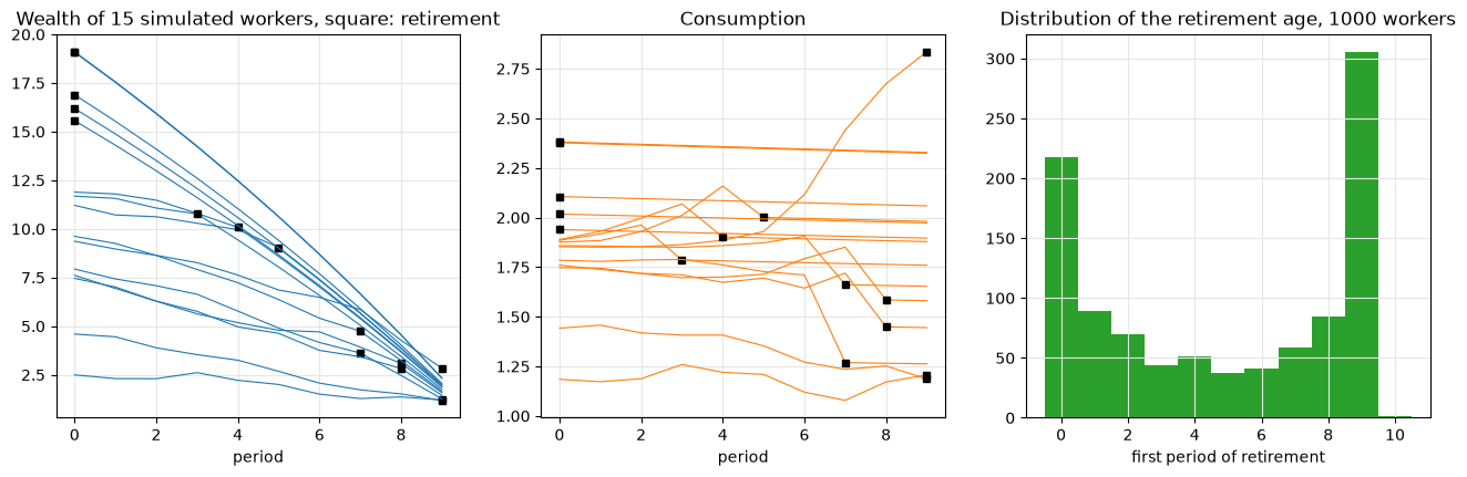

The rich retire in the first period and run their wealth down, the poor work until the last period, where everyone retires: the retirement age distribution is bimodal, driven by initial wealth, with the taste shocks filling the middle. The consumption paths are smooth except for the drop at retirement, the one discontinuity that no shock removes.

Which moments of these simulated data would identify $\delta$ , and which $\sigma$ ?
Keane’s test of Class 16 needs $\beta R = 1$ and no shocks. What does a flat consumption path look like in this model?

Estimation with DC-EGM¶

We can now solve many problems of this type fast, and a fast solver is the inner loop of every estimator:

a fast solver for important problems with discrete and continuous choice allows calibration, structural estimation with your favorite method, and in particular NFXP: the inner loop solves the model, the outer loop optimizes the objective function
the solver can be run repeatedly in some outer loop: for individual heterogeneity, solving the model for each individual in the sample; for unobserved heterogeneity, random effects; and for flexibility in the distributional assumptions

With taste shocks the discrete choices have logit probabilities, so maximum likelihood with discrete and continuous data is straightforward, as in the Monte Carlo experiments of Iskhakov et al. (2017). Without a likelihood, the simulator above is all that the method of simulated moments of the next class needs.

How does EGM as an inner loop compare with MPEC, which avoids the inner loop altogether? Jørgensen (2013) runs the comparison on the infinite horizon Deaton model, maximum likelihood on synthetic data with one structural parameter:

$\beta$		RMSE	Time
0.70	EGM	0.002	0.1 sec
	MPEC	0.049	112.4 sec
0.95	EGM	0.006	1.9 sec
	MPEC	0.009	93.7 sec
0.99	EGM	0.000	5.0 sec
	MPEC	0.000	30.9 sec

Points to take home:

EGM and DC-EGM are fast and accurate solution methods, with no root-finding operations in the regular case and an efficient treatment of the credit constraint
deterministic discrete-continuous problems are hard: kinks in the value functions, discontinuous policy functions, and a snowball effect in the accumulation of kinks over time
with extreme value taste shocks the problem is alleviated; the shocks can be structural or added for smoothing, and they facilitate estimation with discrete choice data

References and additional resources

📖 Iskhakov et al. (2017) “The endogenous grid method for discrete-continuous dynamic choice models with (or without) taste shocks”
📖 Fella (2014) “A Generalized Endogenous Grid Method for Non-Smooth and Non-Concave Problems” — identifies the regions where the Euler equation is not sufficient, and uses VFI inside and EGM outside
📖 Druedahl & Jørgensen (2017) “A general endogenous grid method for multi-dimensional models with non-convexities and constraints” — the upper envelope re-interpolated on a regular grid, in several dimensions
📖 Clausen & Strub (2020) “Reverse Calculus and nested optimization” — the Euler equation remains necessary in discrete-continuous problems
📖 Dobrescu & Shanker (2022) “Fast Upper-Envelope Scan for Discrete-Continuous Dynamic Programming”
📖 Jørgensen (2013) “Structural estimation of continuous choice models: Evaluating the EGM and MPEC”
📖 Carroll (2006) “The method of endogenous gridpoints for solving dynamic stochastic optimization problems”
📄 The dcegm Python package of Maximilian Blesch and coauthors, a JAX implementation of DC-EGM for large models github.com/OpenSourceEconomics/dcegm

References¶

Iskhakov, F., Jørgensen, T., Rust, J., & Schjerning, B. (2017). The endogenous grid method for discrete-continuous dynamic choice models with (or without) taste shocks. Quantitative Economics, 8(2), 317–365. https://doi.org/10.3982/QE643
Clausen, A., & Strub, C. (2020). Reverse Calculus and nested optimization. Journal of Economic Theory, 187, 105019. 10.1016/j.jet.2020.105019
Dobrescu, L. I., & Shanker, A. (2022). Fast Upper-Envelope Scan for Discrete-Continuous Dynamic Programming (Working Paper No. 4181302). SSRN. 10.2139/ssrn.4181302
Druedahl, J., & Jørgensen, T. H. (2017). A general endogenous grid method for multi-dimensional models with non-convexities and constraints. Journal of Economic Dynamics and Control, 74, 87–107. 10.1016/j.jedc.2016.11.005
Jørgensen, T. H. (2013). Structural estimation of continuous choice models: Evaluating the EGM and MPEC. Economics Letters, 119(3), 287–290. 10.1016/j.econlet.2013.02.027
Fella, G. (2014). A generalized endogenous grid method for non-smooth and non-concave problems. Review of Economic Dynamics, 17(2), 329–344. 10.1016/j.red.2013.07.001
Carroll, C. D. (2006). The method of endogenous gridpoints for solving dynamic stochastic optimization problems. Economics Letters, 91(3), 312–320. 10.1016/j.econlet.2005.09.013