📖 Nested fixed point MLE estimation

Tuesday’s solver becomes an estimator once a likelihood is wrapped around it: for every parameter vector, solve the model and evaluate the probability of the data. This class is maximum likelihood for dynamic models, and the nested fixed point (NFXP) algorithm of Rust (1987) that makes it fast.

cd sb-dse-code
git reset --hard HEAD
git pull

Maximum likelihood estimation¶

The maximum likelihood estimator is applicable when the model yields a probability distribution for the observable data. Let $L(z,\theta)$ denote the distribution (pdf) of the observables $z$ implied by the model with parameter vector $\theta$, and let $Z_n = (z_1,\dots,z_n)$ denote the data, consisting of $n$ independent observations, a random sample. MLE and MSM are the two main estimation methods for dynamic economic models, and the method of simulated moments comes later in the course.

Likelihood function¶

If $L(z,\theta)$ is a discrete distribution then $L(z,\theta)$ computed at the data point gives the probability of observing that data point exactly. If $L(z,\theta)$ is a continuous distribution then $L(z,\theta)$ computed at the data point is analogous to the probability of observing it. Either way, independence across observations makes the joint probability of the sample a product,

which is the likelihood function: the data are fixed, and it is a function of the parameters.

The log is there for the numerics as much as for the algebra: a product of a few thousand probabilities underflows to zero long before the sample is exhausted, and a sum of their logs does not. Never take the log of a probability, from Class 6, applies to every term of $\ell_n(\theta)$.

Asymptotic properties of MLE¶

Under regularity conditions the MLE has four properties that make it the default estimator whenever a likelihood is available (Newey & McFadden (1994), Theorems 2.5, 3.3 and 5.1):

1. Consistency: $\hat{\theta}_{MLE} \xrightarrow{p} \theta_0$

2. Asymptotic normality: $\sqrt{n} ( \hat{\theta}_{MLE} - \theta_0 ) \xrightarrow{d} N(0,\mathcal{I}(\theta_0)^{-1})$

3. Asymptotic efficiency: $\mathcal{I}(\theta_0)^{-1}$ is the smallest asymptotic variance attainable in the class of GMM estimators, which includes method of moments and least squares — the large-sample counterpart of the Cramér–Rao bound

4. Functional invariance: the MLE of $\gamma_0 = g(\theta_0)$ is given by $g(\hat{\theta}_{MLE})$ for any function $g(\cdot)$; continuous differentiability of $g$ is needed only for the delta-method standard errors of $\hat{\gamma}$

The price is the regularity conditions — identification, a compact parameter space, continuity and a dominance condition on $\ell(z,\theta)$ for consistency; an interior $\theta_0$, twice differentiability and a nonsingular $\mathcal{I}(\theta_0)$ for normality — and the assumption that the model is correctly specified: a misspecified likelihood still produces an estimate, but the properties above no longer describe it.

Asymptotic variance of the MLE¶

The asymptotic normality result can be read as a statement about the standardized estimator,

where, for a scalar parameter, the variance is given by the inverse of the Fisher information, computed from the pdf $L(z,\theta_0)$ as the expected curvature of the log-likelihood, or equivalently as the expected squared score (under regularity conditions):

The Fisher information matrix can be computed also from the log-likelihood function $\ell_n(\theta_0)$ of $n$ i.i.d. random variables in place of the data $Z_n$, and it scales with the sample size:

Let individual log-likelihoods and scores be

Fisher information can be consistently estimated from a sample of $n$ observations by plugging in the MLE estimate $\hat\theta$ in two different ways:

Newey & McFadden (1994), Theorem 4.4, list mild regularity condition under which both of these estimators are consistent for the true Fisher information $\mathcal{I}(\theta_0)$, leading to

so the standard errors of the estimates are the square roots of the diagonal of the inverse of the negative Hessian of the log-likelihood at the optimum. Every optimizer that uses a Hessian, or an approximation to it, has the standard errors for free.

Outer product of gradients¶

Consider a vector random variable $\tilde{X} = (\tilde{X}_1,\dots,\tilde{X}_K)^{T}$, a column vector $K \times 1$, with expectation given by the $K \times 1$ vector $\mathbb{E}\tilde{X}$. The $K \times K$ variance-covariance matrix $\Sigma$ of $\tilde{X}$ is given by the expectation of the outer product $\otimes$,

The variances of the elements of $\tilde{X}$ are on the main diagonal of $\Sigma$, whereas the off-diagonal elements contain the covariances $cov(\tilde{X}_i,\tilde{X}_j)$ for all $i \ne j$.

Information matrix equality¶

• let $H(\ell_n(\theta_0)) = \frac{\partial^2}{\partial\theta \partial\theta} \ell_n(\theta_0)$ denote the $K \times K$ Hessian matrix of $\ell_n(\theta_0)$

• let $\nabla f(\theta) = \frac{\partial}{\partial\theta} f(\theta)$ denote the gradient of $f(\theta)$, a $K \times 1$ vector, and

• let $\nabla\ell(Z_n, \theta_0) = \big( \frac{\partial}{\partial\theta} \ell(z_1,\theta_0),\dots,\frac{\partial}{\partial\theta} \ell(z_n,\theta_0) \big)$ denote the $K \times n$ matrix of gradients of $\ell(z_i,\theta_0)$ stacked for all $i$.

Then the information matrix equality (Newey & McFadden (1994), Theorem 3.3)

has the sample analogue

The right hand side needs first derivatives only, one score vector per observation. That is what makes it useful inside an optimizer.

Berndt–Hall–Hall–Hausman (BHHH) algorithm¶

The information matrix equality gives an approximation of the Hessian of the log-likelihood function that can be used in a quasi-Newton optimization method,

which is the BHHH algorithm of Berndt et al. (1974), introduced with the other quasi-Newton methods in Class 5. The outer product of gradients is a positive semi-definite matrix for every $\theta$, so even if the approximation is not accurate it never points the Newton iteration in the wrong direction. A search for an appropriate step size in the direction found with the approximated Hessian is part of the algorithm to ensure global convergence.

Where it breaks: the equality holds at $\theta_0$, in expectation, for a correctly specified model. Far from the optimum, in small samples, or under misspecification the outer product is a poor Hessian, and the standard errors it implies are wrong even when the point estimate is fine. The sandwich estimator that combines both sides of the equality, $\hat{\mathcal{J}}_n(\hat\theta)^{-1} \, \nabla\ell(Z_n, \hat\theta) \nabla\ell(Z_n, \hat\theta)^{T} \, \hat{\mathcal{J}}_n(\hat\theta)^{-1}$, is the robust alternative (Newey & McFadden (1994), Section 4.2).

Estimating the bus engine model with NFXP¶

For every value of the structural parameters $\theta = (RC,\theta_1,\theta_{20},\dots,\theta_{2J},\beta)$ we can solve the model fast using NK iterations within the poly-algorithm, and based on the solution $EV_\theta(x,d)$ form the choice probabilities $P(\text{keep}|x,\theta)$ and $P(\text{replace}|x,\theta)$. Given data on mileage $x$ and choices $d$ we can then form the likelihood function and proceed with maximum likelihood estimation.

Data¶

Harold Zurcher kept maintenance records of 162 buses in 8 groups, with monthly observations of the mileage on each bus (the odometer reading) and data on the maintenance operations:

1. Routine periodic maintenance (i.e. brake adjustment)

2. Replacement or repair at the time of failure

3. Major engine overhaul and/or replacement — the focus of the paper

The data are $(x_{i,t},d_{i,t})$, where $x_{i,t}$ is the discretized mileage (bin indexes) and $d_{i,t}$ the observed choice at this mileage for each bus $i$ in each month $t$.

Likelihood function¶

The model delivers two conditional probabilities per observation, the choice given the state and the state transition given the previous state and choice, so

The dependence on $EV_\theta$ is written explicitly because the choice probabilities are a function of the solution of the model, not of $\theta$ directly. The transition part depends on $\theta_2$ only and does not involve the solution at all.

MLE estimator¶

This is an unconstrained optimization, but it requires the computation of $EV_{\theta}$ for each value of the parameter $\theta$ — a fixed point problem inside every function evaluation.

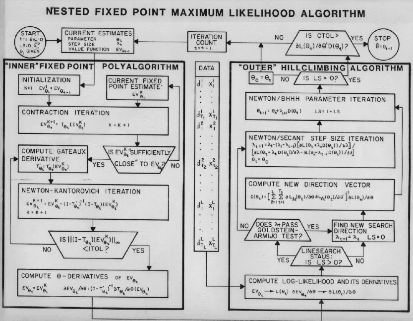
Nested loop¶

The outer loop is a hill-climbing algorithm. The log-likelihood function $\ell_n(\theta,EV_{\theta})$ is maximized with respect to $\theta$ by a quasi-Newton algorithm with the BHHH approximation of the Hessian, and each evaluation of $\ell_n(\theta,EV_{\theta})$ requires the solution for the fixed point $EV_{\theta}$.

The inner loop is the fixed point algorithm: the solver for the fixed point of the Bellman operator $EV_{\theta} = \Gamma(EV_{\theta})$, successive approximations (VFI) plus Newton–Kantorovich iterations in the poly-algorithm of Tuesday.

Important details¶

1. Performance: a gradient based Newton method to maximize the likelihood

2. Analytical gradients: using the implicit function theorem and the chain rule for the outer loop, and the Fréchet derivative for the inner loop

3. Use BHHH: the outer product of gradients approximation for the Hessian

4. Numerical stability: recenter the logsum and the choice probabilities, the de-maxing trick of Class 6

5. Further info: the NFXP manual, see the references below

Each of these is a difference between an estimator that runs in seconds and one that runs overnight. The comparison in Iskhakov et al. (2016) is exactly the difference between an NFXP with items 1–3 and one without.

Analytical gradient of the likelihood function¶

Differentiating the log-likelihood term by term,

is straightforward with multiple applications of the chain rule. The key point is expressing the derivatives of the expected value function $\frac{\partial EV_{\theta}}{\partial \theta}$, which is done with the Banach space version of the implicit function theorem applied to the fixed point equation:

Here $\Gamma_{\theta}(\cdot)$ is the finite approximation of the Bellman operator in expected value function space, and $\frac{\partial \Gamma_{\theta}}{\partial EV_{\theta}}$ is the finite approximation of its Fréchet derivative — the same matrix the NK step already computes and factorizes. The gradient of the likelihood is therefore nearly free once the model is solved by NK: one more solve with the same matrix and a different right hand side.

📖 John Rust “NFXP Pocket Guide” Download pdf

Replication of Rust (1987)¶

The estimator is in the folder session10-11/ of the code repository: nfxp.py is the model class of Tuesday with the data attached and the likelihood, its analytical score and BHHH on top, and the notebook replicate_rust1987.ipynb runs everything shown below. Run on Harold Zurcher’s records for bus groups 1–4, on the 175-cell mileage grid of the paper and with $\beta = 0.9999$:

from nfxp import read_busdata, estim_zurcher

data = read_busdata()                       # groups 1-4, 175 cells, Rust's cell convention
est = estim_zurcher(data)                   # the model with the data attached
result = est.estimate()                     # frequencies, then (RC, c), then everything
print(result)

NFXP estimates, beta = 0.9999, n = 175, N = 8156 bus-months
method bhhh, converged True, 0.066 s, 82 inner solves, 262 inner iterations
parameter     estimate        s.e.
RC             9.76867     1.22629
c              1.34283     0.31532
p0             0.10705     0.00343
p1             0.51522     0.00554
p2             0.36216     0.00532
p3             0.01434     0.00132
p4             0.00086     0.00032
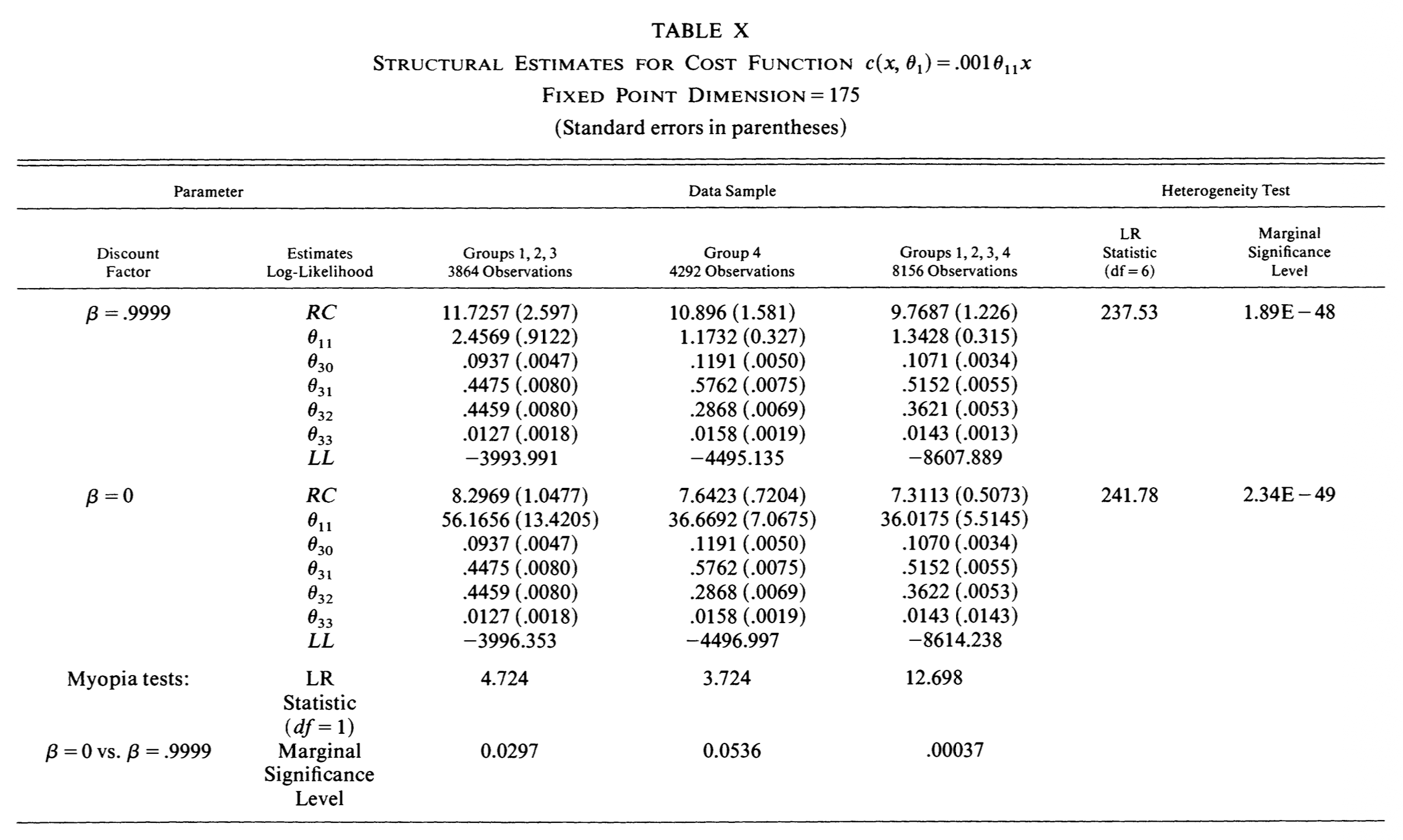
log-likelihood -8607.8894

These are the numbers of the last row of Table X in Rust (1987) ($\theta_{11}$ is c, $\theta_{30},\dots,\theta_{33}$ are the first four transition probabilities):

The same estimator on each of the six samples of the table:

for beta in (0.9999, 0.0):
    for groups in ((1, 2, 3), (4,), (1, 2, 3, 4)):
        r = estim_zurcher(read_busdata(groups=groups), beta=beta).estimate()
        print(beta, groups, r.N, r.theta[:2], r.se[:2], r.loglik, r.theta[2:6])

  beta groups        N       RC    (se)        c      (se)     loglik  transition probabilities
0.9999 1,2,3      3864  11.7257   2.597   2.4569    0.9122  -3993.991  0.0937 0.4475 0.4459 0.0127
0.9999 4          4292  10.0896   1.581   1.1732    0.3265  -4495.135  0.1191 0.5762 0.2868 0.0158
0.9999 1,2,3,4    8156   9.7687   1.226   1.3428    0.3153  -8607.889  0.1071 0.5152 0.3622 0.0143
   0.0 1,2,3      3864   8.2969   1.048  56.1656   13.4205  -3996.353  0.0937 0.4475 0.4459 0.0127
   0.0 4          4292   7.6423   0.720  36.6692    7.0675  -4496.997  0.1191 0.5762 0.2868 0.0158
   0.0 1,2,3,4    8156   7.3113   0.507  36.0175    5.5145  -8614.238  0.1070 0.5152 0.3622 0.0143

Every entry replicates at the precision of the paper, once the data are read the way Rust’s code read them: mileage cell $k = \lceil x \cdot 175 / 450000 \rceil$ used as a one-based index, so that the decision is evaluated at grid point $k-1$ and the transition after a replacement is recorded from cell 0 to cell $k$, one cell more than the model’s own reset. The one exception is $RC$ for group 4 at $\beta = .9999$, which the paper prints as 10.896 for 10.0896: every other number in that row agrees. Two things to notice in the myopic rows: the cost parameter is nearly thirty times larger when the future is not counted, and the log-likelihood is lower by 6.3, the paper’s test of myopia.

Counterfactuals¶

The estimates describe Zurcher’s behavior only through the model. What that behavior implies for the fleet is the ergodic distribution of mileage under the estimated replacement policy, against the mileage actually observed:

_, pk, _ = est.solve()                             # the policy at the estimates
q, q_keep, q_replace = ergodic_distribution(est, pk)   # defined in replicate_rust1987.ipynb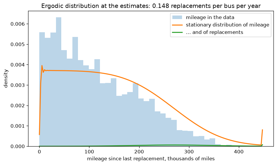

The data sit to the left of the stationary distribution: most buses enter the sample with a new engine, and the panel is too short to reach the steady state. The counterfactual that the paper is after is the demand for engine replacement as a function of its price, obtained by re-solving the model on a grid of $RC$ and reading the replacement rate off the ergodic distribution each time. Converting $RC$ into dollars with the average replacement cost of $8062 for these groups (Table III of the paper) gives Figure 7 of the paper, for the dynamic and the myopic estimates:

RC_grid = np.linspace(0.5, 30, 60)                 # demand_curve() is in the notebook too
myopic = estim_zurcher(data, beta=0.0)
myopic.estimate()                                  # the myopic model, re-estimated
for m in (est, myopic):
    scale = 8062 / m.RC                            # dollars per unit of RC at the estimate
    plt.plot(RC_grid * scale, demand_curve(m, RC_grid), label=f'beta = {m.beta}')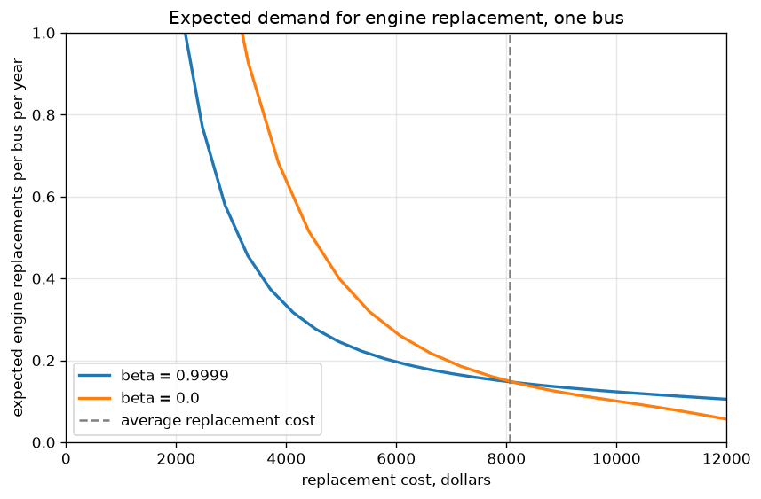

The two models fit the data equally well at the observed price and disagree everywhere else: the myopic bus manager reacts to a price change far more, because in his model the only reason to replace is today’s cost. This is why the discount factor matters for policy even when the likelihood can barely tell $\beta = 0.9999$ from $\beta = 0$. A known issue: the demand curves do not exactly replicate Figure 7 of the paper, although the estimates they are computed from reproduction of its tables.