📖 The endogenous gridpoint method

Every solver of Class 16 solves a nonlinear problem in every state on every iteration, a maximization or a root of the Euler equation. The endogenous gridpoint method of Carroll (2006) turns the problem around: fix the choice, and find the state in which it is optimal. For the consumption-savings model this needs no optimization and no root finding at all.

Running the code for this lecture

The code for this class is in the folder session17-oct22/ of the course code repository. It reuses the model and the solvers of Class 16, collected in the module deaton.py in the same folder.

You should have cloned that repository already — if not, the instructions are in the algorithms and complexity lecture.

Update your copy before the class. Editing a file in place makes git pull refuse to update it, so discard whatever you changed while experimenting:

cd sb-dse-code
git reset --hard HEAD
git pull

Nothing in this repository is submitted, so experiment freely — but copy anything you want to keep out of it first, or commit that to a branch of your own.

Setting up the Python environment is covered in Python.

Homework kappa_floor: EGM with a consumption floor

Graded homework: task kappa_floor in the class repository. Collect it and work on a copy in your own repository:

git pull upstream main                          # collect the task
cp -r tasks/kappa_floor solutions/kappa_floor   # work on the copy

Add a government consumption floor to the consumption-savings model with deterministic income, and solve it with value function iterations with discretized choice and with the EGM solver of this class. Compare the two solutions for several levels of the floor, and explain what you find.

The notebook floor.ipynb in the task folder carries the details of the task, step by step.

Submit it as a pull request, following the git workflow. One of you presents a solution at the start of the next Tuesday class.

The idea on cake eating¶

Take the cake eating problem. The first order condition for $c_t$ and the envelope theorem,

u'(c_t) = \beta V'(W_{t+1}), \qquad V'(W_t) = \beta V'(W_{t+1}),

combine into $V'(W_t) = u'(c_t)$ at every $t$ , and into the Euler equation

\frac{1}{c_t} = \frac{\beta}{c_{t+1}} \quad\Leftrightarrow\quad c_t = \frac{c_{t+1}}{\beta}

Read it backwards: given what is left for the future, $A = W - c$ , and the policy for next period, the Euler equation gives today’s consumption in closed form, and the budget gives the cake size at which that consumption is optimal, $W = A + c$ .

Value function iterations and time iterations fix a grid on the state $W$ and search for the optimal $c$ at every point. What does the search cost?

Time: an iterative optimizer or root finder runs in every point of the state space, on every iteration
Accuracy: the wealth level where the borrowing constraint starts to bind is almost never a point of the fixed grid, so the kink of the policy is smeared between two grid points
Reliability: a global maximum is hard to guarantee once the problem is not concave

The endogenous gridpoint method (EGM) fixes a grid on the post-decision state $A$ instead, computes $c$ directly, and lets the grid on the state come out of the computation, endogenously:

Algorithm (EGM for the cake eating problem)

Input: a grid $0 \leqslant A_1 < \dots < A_n$ on the post-decision state, the initial policy $c_0(W) = W$ , and a tolerance $\epsilon > 0$ .

Iterate for $i = 1, 2, \dots$ :

For every grid point $A_j$ , $j = 1, \dots, n$ :
1. next period cake: $W'_j = A_j$
2. next period consumption from the previous policy: $c'_j = c_{i-1}(W'_j)$
3. current consumption from the inverted Euler equation: $c_j = c'_j / \beta$
4. the endogenous grid point: $W_j = A_j + c_j$
Let $c_i(W)$ be the linear interpolation of the points $(W_j, c_j)$ , $j = 1, \dots, n$ .
Stop if $\lVert c_i - c_{i-1} \rVert_\infty < \epsilon$ , otherwise continue with $i + 1$ .

Output: the policy function $c(W) = c_i(W)$ .

There is no maximization and no root finding, only function evaluations. And the Euler equation holds exactly at the endogenous grid points, so the method is as accurate as time iterations at a fraction of the cost.

The endogenous grid points $W_j$ change from one iteration to the next. Is that not a problem?
Which step of the algorithm would need a root finder if the utility function was more complex than $\log(c)$ ?

Consumption-savings with random returns (Phelps)¶

Cake eating with a return on savings is the model of Phelps (1962). The consumer has no income and invests all savings in an asset with a random return:

V_t(M_t) = \max_{0 \leqslant c \leqslant M_t} \Big\{ u(c) + \beta\, \mathbb{E}\, V_{t+1}\big(\tilde R\, (M_t - c)\big) \Big\}, \qquad u(c) = \frac{c^\rho - 1}{\rho}

$M_t$ is cash on hand, all resources available in period $t$
$A_t = M_t - c_t$ are the savings at the end of period $t$
$\tilde R$ is the gross return on savings, random (marked by tilde), independent over time
$\rho < 1$ is the exponent of the utility function, the coefficient of relative risk aversion is $1 - \rho$ , and $u(c) \to \log c$ as $\rho \to 0$
the horizon is finite, and in the last period the consumer eats everything, $c_T(M) = M$

The solution is analytical Hakansson, 1970. With $t$ periods to go, the policy is linear in wealth:

c_{T-t}(M) = M \Big( \sum_{i=0}^{t} K^i \Big)^{-1}, \qquad K = \big( \beta\, \mathbb{E}\, \tilde R^{\rho} \big)^{\frac{1}{1-\rho}}

and the value function is a power of wealth:

V_{T-t}(M) = \frac{M^\rho}{\rho} \Big( \sum_{i=0}^{t} K^i \Big)^{1-\rho} - \frac{1}{\rho} \sum_{i=0}^{t} \beta^i

In the logarithmic case $K \to \beta$ , so $c_{T-t}(M) = M\,(1-\beta)/(1-\beta^{t+1})$ and $V_{T-t}(M) = \log(M) \sum_{i=0}^{t} \beta^i + K_t$ , with $K_t$ a constant that depends on the primitives.

As $t \to \infty$ the policy tends to $c(M) = (1-\beta) M$ , the cake eating solution, whatever the return.

Verification for one period

In period $T-1$ , with $c_T(M) = M$ , the first order condition for $c$ is

c^{\rho-1} = \beta\, \mathbb{E}\big[\tilde R^{\rho}\big] (M - c)^{\rho-1} = K^{1-\rho} (M - c)^{\rho-1},

so $c / (M - c) = 1/K$ and $c_{T-1}(M) = M/(1+K)$ .

Substituting $c$ and $M - c = MK/(1+K)$ into the Bellman equation,

V_{T-1}(M) = \frac{c^\rho + K^{1-\rho} (M-c)^\rho}{\rho} - \frac{1+\beta}{\rho} = \frac{M^\rho}{\rho} (1+K)^{1-\rho} - \frac{1+\beta}{\rho},

which is the formula with $t = 1$ . Induction on $t$ repeats the same steps.

Why is the solution so simple?

utility is homothetic, and wealth next period is proportional to savings, so the problem scales: doubling $M$ doubles the optimal $c$
the random return multiplies all of next period’s wealth, so it changes the share consumed through $K$ , not the shape of the policy

Is this finite or infinite horizon problem?
How does the share of wealth consumed change as the end of the horizon approaches?
With log utility the policy does not depend on the distribution of $\tilde R$ at all. Why?

EGM for the consumption-savings model (Deaton)¶

Adding income $y$ breaks the simple structure: next period wealth $\tilde R A + y$ is no longer proportional to savings, the borrowing constraint starts to bind for low wealth.

No closed form solution!

See Carroll & Kimball (1996) for the discussion of all special cases.

In the model of Deaton (1991) the Euler equation holds with an expectation over income, and the post-decision state is savings

A = M - c,

u'\big(c(M)\big) = \beta R\, \mathbb{E}_{y}\, u'\big(c(RA + \tilde{y})\big)

Savings $A$ determine everything on the right-hand side:

next period wealth $M' = RA + \tilde y$ for every income draw and,
through next period’s policy, the expected marginal utility.

So for a given policy $c(\cdot)$ , every value of $A$ gives one point of the updated policy as a parameterized curve $(M(A), c(A))$ defined by

\begin{cases} c = (u')^{-1}\Big( \beta R\, \mathbb{E}_{y}\, u'\big(c(RA + \tilde{y})\big) \Big) \\[4pt] M = A + c \end{cases}

Let’s stop here for a moment..

Example: parameterized curves

A parameterized curve is the set of points $\big(x(t), y(t)\big)$ traced as the parameter $t$ runs over an interval: both coordinates are functions of $t$ , and neither has to be a function of the other.

The circle $x(t) = \cos t$ , $y(t) = \sin t$ , $t \in [0, 3\pi/2]$ , is the textbook example. It is not the graph of a function: some $x$ have two points on the curve.
The EGM step has savings $A$ as the parameter and the coordinates $M(A) = A + c(A)$ and $c(A)$ . Because $M(A)$ is increasing in $A$ , every $M$ has exactly one point on the curve, and the curve is the graph of the policy function $c(M)$ .

The figure marks equally spaced values of the parameter on both curves, with an illustrative increasing $c(A)$ on the right.

import numpy as np
import matplotlib.pyplot as plt

fig, (ax1, ax2) = plt.subplots(1, 2, figsize=(12, 4.8))
t = np.linspace(0, 1.5 * np.pi, 200)                      # the parameter, dense for the curve
tk = np.linspace(0, 1.5 * np.pi, 7)                        # a few marked values of the parameter
ax1.plot(np.cos(t), np.sin(t), 'C0-')
ax1.plot(np.cos(tk), np.sin(tk), 'C0o')
for v in tk:
    ax1.annotate(f't = {v / np.pi:.2g}π', (np.cos(v), np.sin(v)), textcoords='offset points', xytext=(8, 4))
ax1.set(xlabel='x(t) = cos t', ylabel='y(t) = sin t', title='Generic parameterized curve', aspect='equal')

A = np.linspace(0, 8, 200)                                 # the parameter: savings
Ak = np.linspace(0, 8, 9)                                  # equally spaced grid on savings
c = lambda A: 1 + 1.2 * np.sqrt(A)                         # an illustrative increasing consumption
ax2.plot(A + c(A), c(A), 'C1-')
ax2.plot(Ak + c(Ak), c(Ak), 'C1o')
for a in Ak[::2]:
    ax2.annotate(f'A = {a:g}', (a + c(a), c(a)), textcoords='offset points', xytext=(-10, 8))
ax2.plot(Ak + c(Ak), np.zeros_like(Ak), 'k|', ms=12)       # the endogenous grid on wealth
ax2.set(xlabel='wealth M(A) = A + c(A)', ylabel='consumption c(A)', ylim=(-0.3, 5),
        title='EGM: the policy as a curve parameterized by savings')
for ax in (ax1, ax2):
    ax.grid(color='0.9')
plt.show()

On the right the points are equally spaced in $A$ but not in $M$ : the ticks on the horizontal axis are the endogenous grid.

Ok, back to consumption and savings..

Let $A$ be a parameter, and consider the parameterized curve $(M,c)$

\begin{cases} c = (u')^{-1}\Big( \beta R\, \mathbb{E}_{y}\, u'\big(\check{c}(RA + \tilde{y})\big) \Big) \\[4pt] M = A + (u')^{-1}\Big( \beta R\, \mathbb{E}_{y}\, u'\big(\check{c}(RA + \tilde{y})\big) \Big) \end{cases}

Here $\check{c}(\cdot)$ is the policy from the previous iteration of the backward induction or VFI, and is ``known’', approximated by interpolation on the previous iteration endogenous grid over $M$ .

With $u(c) = \log c$ the inverse marginal utility is $(u')^{-1}(x) = 1/x$

The expectation can be computed by quadrature, it is then a weighted sum over the income nodes.

Endogenous gridpoint method (EGM) step

Given (an estimate of) a policy function $c(\cdot)$ , the EGM step maps a point $A_j$ from the grid on savings and into the points $(M_j, c_j)$ of the updated policy:

next period wealth in every income node: $M'_{jk} = R A_j + y_k$
next period consumption from the current policy: $c'_{jk} = c(M'_{jk})$
the expected marginal utility, by quadrature: $\mathbb{E}u'_j = \sum_k \omega_k\, u'(c'_{jk})$
current consumption from the inverted Euler equation: $c_j = (u')^{-1}(\beta R\, \mathbb{E}u'_j)$
the endogenous grid point: $M_j = A_j + c_j$

The EGM iterations repeat the step, interpolating the points $(M_j, c_j)$ into the policy for the next step, until the policy stops changing.

Algorithm (EGM in the infinite horizon)

Input: a grid $0 = A_1 < A_2 < \dots < A_n$ on savings, quadrature nodes and weights $(y_k, \omega_k)$ , $k = 1, \dots, K$ , for the income, the initial policy $c_0(M) = M$ , and a tolerance $\epsilon > 0$ .

Iterate for $i = 1, 2, \dots$ :

For every grid point $A_j$ , $j = 1, \dots, n$ , take the EGM step with the policy $c_{i-1}$ to recover $(M_j, c_j), j=1,\dots,n$
Add the origin $(M, c) = (0, 0)$ to the points $(M_j, c_j)$ , for the credit constrained region $M < M_1$
Let $c_i(M)$ be the linear interpolation of these $n + 1$ points
Stop if $\lVert c_i - c_{i-1} \rVert_\infty < \epsilon$ on the latest endogenous grid, otherwise continue with $i + 1$

Output: the policy function $c(M) = c_i(M)$ , given by the points of the last endogenous grid.

In a finite horizon model the same step runs backward in time. The last period policy is $c_T(M) = M$ , and each EGM step returns the policy one period earlier. Starting the infinite horizon iterations from $c_0(M) = M$ is the same backward induction, so iteration $i$ is the policy $i$ periods before the end.

The figure below shows the first iterations on a grid of only five points, starting from the policy $c_0(M) = M$ , defined by two points: the consumer eats everything.

import numpy as np
import matplotlib.pyplot as plt

def lin(x, xp, fp):
    '''Linear interpolation, extrapolated linearly beyond the last point'''
    slope = (fp[-1] - fp[-2]) / (xp[-1] - xp[-2])
    return np.where(x > xp[-1], fp[-1] + slope * (x - xp[-1]), np.interp(x, xp, fp))

def egm_iterations(beta, R, y, K, A=np.linspace(0, 10, 5), origin=False, title=''):
    '''Plot the first K iterations of EGM with log utility and deterministic income y'''
    M0, c0 = np.array([0., 10.]), np.array([0., 10.])     # initial policy: consume everything
    fig, ax = plt.subplots(1, 3, figsize=(14, 4.2))
    ax[2].plot(M0, c0, 'o-', ms=4, lw=0.8, label='iteration 0')
    for i in range(1, K + 1):
        c1 = np.maximum(lin(R * A + y, M0, c0), 1e-10)    # next period consumption, kept positive
        c = c1 / (beta * R)                               # inverted Euler equation: 1/c = beta R / c1
        M = A + c                                         # endogenous grid points
        if origin:                                        # add the origin: the constrained segment
            M, c, Ap = np.r_[0, M], np.r_[0, c], np.r_[np.nan, A]
        else:
            Ap = A
        for k, (x, yy) in enumerate(((Ap, c), (Ap, M), (M, c))):
            ax[k].plot(x, yy, 'o-', ms=4, lw=0.8, label=f'iteration {i}')
        M0, c0 = M, c
    for a, (xl, t) in zip(ax, (('savings A', 'consumption c(A)'), ('savings A', 'wealth M(A)'),
                                ('wealth M', 'consumption c(M)'))):
        a.set(xlabel=xl, title=t); a.grid(color='0.9')
    ax[2].legend(fontsize=8)
    fig.suptitle(title)
    plt.show()

egm_iterations(beta=0.95, R=1.0, y=0.0, K=4, title='Cake eating, beta = 0.95, R = 1, y = 0')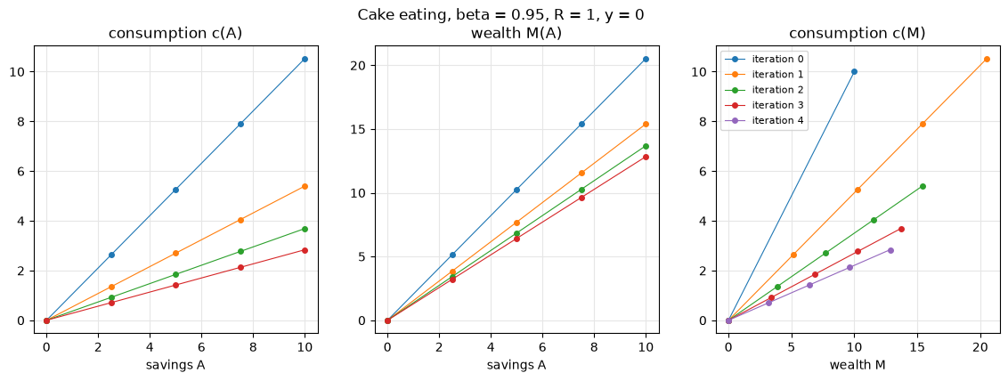

Each iteration produces five points of the policy, and the points move: the grid on $M$ is a product of the iteration, while the grid on $A$ stays put.

Corner solutions¶

The EGM step uses the Euler equation, which holds only at interior solutions!

The constraint $0 \leqslant c \leqslant M$ needs separate care.

The lower bound $c \geqslant 0$ never binds when $\lim_{c \to 0} u(c) = -\infty$ , which holds for $\log c$ and for any CRRA utility with $\rho \geqslant 1$ , or any other utility under the Inada conditions. Handy! Don't need to worry about lower bound in most applications
The upper bound $c \leqslant M$ binds when the consumer would like to borrow, and then $A = 0$ . Handy!! We control the grid on A!

So, to enforce the constraint, we simply ensure that the exogenous grid on $A$ satisfies $A \geqslant 0$ .

What does EGM step return for $A=0$ ?

Many but unfortunately not all application are subject to the following theorem

The EGM step at $A_1 = 0$ gives the largest wealth at which saving nothing is optimal,

M_1 = (u')^{-1}\Big( \beta R\, \mathbb{E}_{y}\, u'\big(c(\tilde{y})\big) \Big),

and for every $M < M_1$ the consumer must also save nothing: the constraint binds and $c(M) = M$ .

In the code this is one extra point at the origin, $(M, c) = (0, 0)$ : linear interpolation between it and $(M_1, c_1)$ is exactly the 45-degree segment $c = M$ .

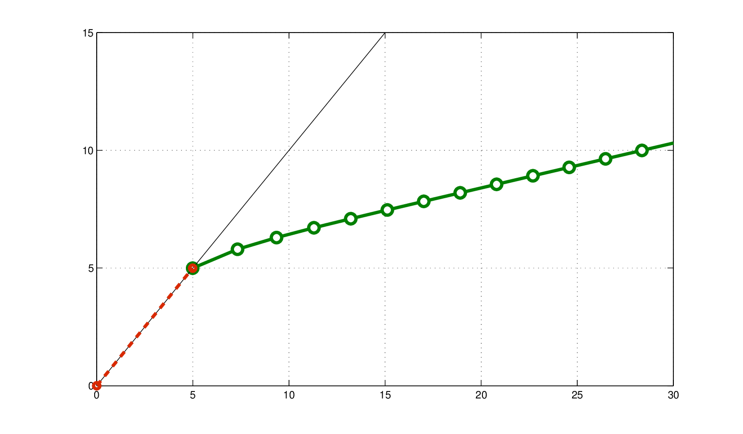
The kink of the policy is located exactly, at an endogenous grid point, and not smeared between two points of a fixed grid as with VFI or time iterations.

This greatly benefits the accuracy of EGM for all the cases where the wealth level in the data/simulation is near the kink of the policy function.

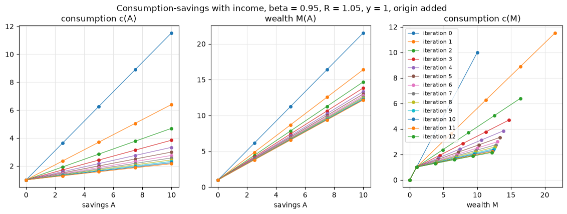
With income, the consumer with little wealth eats all of it and waits for the next paycheck, and the policy has a kink where the constraint stops binding. Without the point at the origin, the interpolated policy below $M_1$ would be an extrapolation of the interior solution, and the consumer would be allowed to borrow.

Why does the grid on savings start at $A = 0$ , and what would a grid point $A < 0$ mean?
The kink of the policy at $M_1$ moves from one iteration to the next. How do VFI and time iterations on a fixed grid represent such a kink?

Implementation and comparison¶

The EGM solver for the stochastic model is a few lines, fully vectorized: savings along the first axis, income nodes along the second, and the expectation as a product with the weights. It uses the model object and the tools of Class 16, from the module deaton.py.

import sys, time, pathlib, tempfile, urllib.request
CODE = pathlib.Path('../gh-code/session17-oct22')          # the code of Class 16, collected in deaton.py
if not CODE.exists():                                     # otherwise fetch it from the code repository
    CODE = pathlib.Path(tempfile.mkdtemp())
    urllib.request.urlretrieve('https://raw.githubusercontent.com/fediskhakov/sb-dse-code/main/session17-oct22/deaton.py',
                               CODE / 'deaton.py')
sys.path.insert(0, str(CODE))
import deaton                                             # model object and solvers of Class 16

def solve_egm(m, maxiter=500, tol=1e-4, callback=None):
    '''EGM for the consumption-savings model, returns the policy on the state grid m.grid'''
    A = np.linspace(0, m.Mbar, m.ngrid)                   # grid on savings, the post-decision state
    M0, c0 = np.array([0., m.Mbar]), np.array([0., m.Mbar])   # initial policy: consume everything
    for i in range(maxiter):
        M1 = m.next_wealth(A[:, None], 0, m.quadp[None, :])   # next period wealth: savings x income nodes
        c1 = np.maximum(deaton.interp(M1, M0, c0), m.eps) # next period consumption, kept positive
        rhs = m.beta * m.R * (m.mu(c1) @ m.quadw)         # RHS of the Euler equation
        c = np.r_[0., m.imu(rhs)]                         # inverted Euler equation, origin added
        M = np.r_[0., A + c[1:]]                          # endogenous grid points
        err = np.max(np.abs(deaton.interp(m.grid, M, c) - deaton.interp(m.grid, M0, c0)))
        if callback: callback(iter=i, M=M, c=c, err=err)
        if err < tol: break
        M0, c0 = M, c
    else:
        raise RuntimeError('No convergence: maximum number of iterations achieved')
    return deaton.interp(m.grid, M, c)                    # policy on the fixed grid, to compare

The policy is returned on the fixed state grid of the model, so all four solvers can be compared with the same Euler residuals.

The experiments below use the defaults of the model object of Class 16, unless stated otherwise:


discount factor	$\beta = 0.9$
gross return	$R = 1.05$
income	log-normal, $\log \tilde y \sim N(0, \sigma^2)$ , $\sigma = 0.5$
utility	$u(c) = \log c$
state grid	100 equally spaced points on $(0, \overline{M}]$ , $\overline{M} = 10$
choice grid, discretized VFI	250 shares of wealth on $(0, 1]$
savings grid, EGM	100 equally spaced points on $[0, \overline{M}]$
quadrature	10 Gauss–Hermite nodes, the default of `deaton.py` (`quad='legendre'` gives Gauss–Legendre on the CDF, as in Class 16)
tolerance	10^-4 for the convergence plots, 10^-12 for the comparisons
grid sizes in the comparisons	6 sizes from 50 to 500 points, equally spaced in logs, on the state grid, and the same number on the savings grid of EGM; the choice grid stays at 250
Phelps test	no income, $R = 1.05$

Convergence of the four solvers¶

The figure shows every iteration of the four solvers on the model of Class 16, from consuming everything to convergence at the tolerance 10^-4, darker to lighter.

m = deaton.deaton()                                       # beta = 0.9, R = 1.05, sigma = 0.5, 100 points
runs = {'VFI, discretized choice': lambda cb: deaton.solve_vfi(m, deaton.bellman_discretized, callback=cb),
        'VFI, continuous choice': lambda cb: deaton.solve_vfi(m, deaton.bellman_continuous, callback=cb),
        'time iterations': lambda cb: deaton.solve_timeiter(m, callback=cb),
        'EGM': lambda cb: solve_egm(m, callback=cb)}
fig, axes = plt.subplots(2, 2, figsize=(14, 10), sharex=True, sharey=True)
for ax, (name, run) in zip(axes.ravel(), runs.items()):
    iters = []                                            # the callback collects the policy of every iteration
    def collect(**kw):
        iters.append((m.grid, kw['policy']) if 'policy' in kw else (kw['M'], kw['c']))   # EGM: endogenous grid
    run(collect)
    for (M, c), col in zip(iters, plt.cm.viridis(np.linspace(0, 1, len(iters)))):
        ax.plot(M, c, color=col, lw=0.8)
    ax.plot(*iters[-1], 'k-', lw=2, label=f'converged after {len(iters)} iterations')
    ax.plot(m.grid, m.grid, 'k:', lw=0.8)
    ax.set(title=name, xlim=(0, m.Mbar), ylim=(0, 3.5))
    ax.grid(color='0.9'); ax.legend(loc='lower right')
for ax in axes[1]: ax.set(xlabel='wealth M')
for ax in axes[:, 0]: ax.set(ylabel='consumption c')
plt.tight_layout(); plt.show()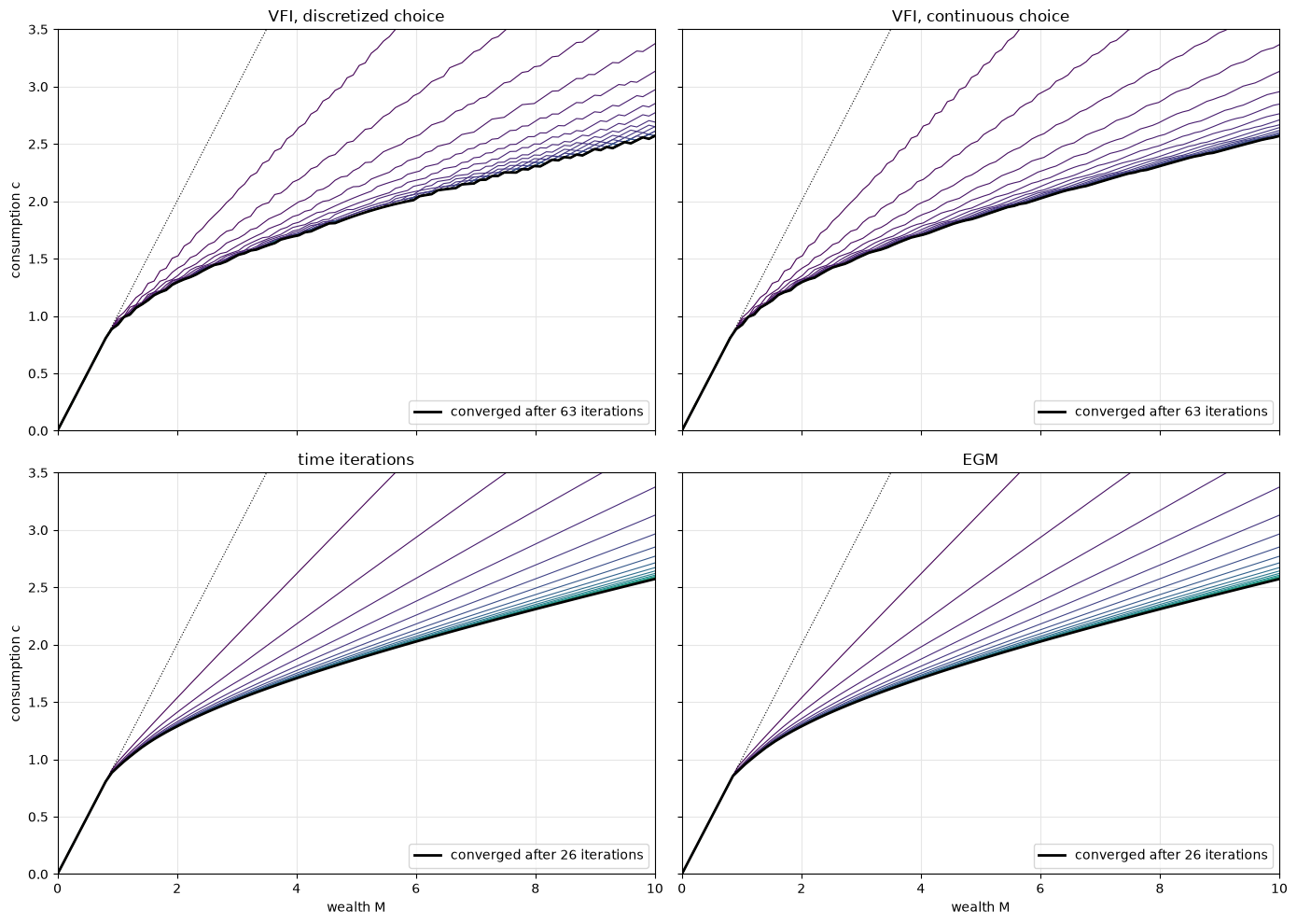

All four arrive at the same policy. VFI needs 63 iterations, at the rate $\beta$ of the contraction of the Bellman operator, time iterations and EGM about 26. An EGM iteration is also the cheapest: no optimizer and no root finder, only interpolation and arithmetic.

Accuracy and speed as the grid grows¶

Each solver now runs on 6 grids from 50 to 500 points with the tight tolerance 10^-12, so that what we measure is the error of the grid and not of the stopping rule. The figure shows the Euler residuals and the run time on the model with income risk, $\sigma = 0.5$ . A solver that does not reach the tolerance within 2000 iterations would be left out of the plot for that grid.

tol, maxiter = 1e-12, 2000
solvers = {'VFI, discretized choice': lambda m: deaton.solve_vfi(m, deaton.bellman_discretized, tol=tol, maxiter=maxiter),
           'VFI, continuous choice': lambda m: deaton.solve_vfi(m, deaton.bellman_continuous, tol=tol, maxiter=maxiter),
           'time iterations': lambda m: deaton.solve_timeiter(m, tol=tol, maxiter=maxiter),
           'EGM': lambda m: solve_egm(m, tol=tol, maxiter=maxiter)}
grids = np.unique(np.geomspace(50, 500, 6).round().astype(int))    # 6 grid sizes, equally spaced in logs
def attempt(solve, m):
    '''Solve the model, or return None if the solver does not converge within maxiter'''
    try:
        return solve(m)
    except RuntimeError:
        return None

res = {name: {'euler': [], 'time': []} for name in solvers}
for name, solve in solvers.items():
    for n in grids:
        m = deaton.deaton(ngrid=n)                        # income risk, sigma = 0.5
        t0 = time.perf_counter()
        c = attempt(solve, m)
        res[name]['time'].append(np.nan if c is None else time.perf_counter() - t0)
        res[name]['euler'].append(np.nan if c is None else deaton.accuracy(m, c))

titles = {'euler': 'Mean |relative Euler residual|, σ = 0.5',
          'time': 'Run time in seconds, σ = 0.5'}
fig, axes = plt.subplots(2, 1, figsize=(12, 10))
for ax, (key, title) in zip(axes, titles.items()):
    for name in solvers:
        ax.plot(grids, res[name][key], 'o-', label=name)
    ax.set(xscale='log', yscale='log', xlabel='grid points', title=title)
    ax.set_xticks(grids, [str(n) for n in grids]); ax.minorticks_off()
    ax.grid(color='0.9'); ax.legend()
plt.tight_layout(); plt.show()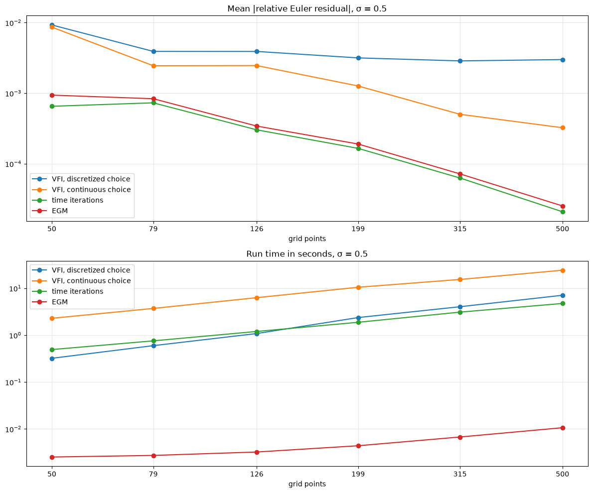

Euler residuals: EGM and time iterations are the most accurate and improve fastest with the grid, to a few times 10^-5 on the finest grid. VFI with continuous choice follows, and the discretized solver stalls at a few times 10^-3, capped by its choice grid.
Run time: EGM takes from 2 to 15 milliseconds, two to three orders of magnitude less than the other three, whose run time grows linearly with the grid.

EGM is as accurate as time iterations, the most accurate of the earlier solvers, at a tiny fraction of the cost. All of the speed comes from replacing the search in every state by a closed-form inversion of the Euler equation.

How EGM compares to the analytical solution¶

The deterministic Phelps model with log utility, no income and a fixed return $R$ has the analytical policy $c(M) = (1-\beta) M$ in the infinite horizon. The model object of Class 16 covers it once the income nodes are set to zero. The table reports the largest absolute difference between the EGM policy and the analytical one on the grid.

print(f'{"grid":>5} {"max |c(M) - (1 - beta) M|":>27}')
for n in grids:
    m = deaton.deaton(ngrid=n, nquad=2)
    m.quadp = np.zeros(2)                                 # no income: the deterministic Phelps model
    c = solve_egm(m, tol=tol, maxiter=maxiter)
    print(f'{n:>5} {np.max(np.abs(c - (1 - m.beta) * m.grid)):>27.2e}')

 grid   max |c(M) - (1 - beta) M|
   50                    8.45e-12
   79                    8.45e-12
  126                    8.45e-12
  199                    8.45e-12
  315                    8.45e-12
  500                    8.45e-12

EGM reproduces the analytical policy to about 10^-11 on every grid, the precision of the stopping rule, not of the grid. The policy is linear in wealth, and linear interpolation reproduces it without error.

The class of models EGM solves¶

EGM in this form solves problems with one continuous state, wealth $M$ , one continuous choice, consumption $c$ , and possibly exogenous states $s$ :

V(M, s) = \max_{0 \leqslant c \leqslant M} \Big\{ u(c) + \beta\, \mathbb{E}\big[ V(M', s') \,\big|\, s \big] \Big\}, \qquad A = M - c, \qquad M' = f(A, s', \tilde\xi')

with the following properties:

utility: $u'(c) > 0$ and $u''(c) < 0$ , and the inverse marginal utility $(u')^{-1}$ has an analytical form
post-decision state: next period wealth depends on $(M, c)$ only through savings $A = M - c$ , by a differentiable function $f$ with $\partial f / \partial A > 0$ ; in the Deaton model $f = RA + \tilde y$ , in the Phelps model $f = \tilde R A$
exogenous states: $P(s' \mid M, s) = P(s' \mid s)$
constraint: $0 \leqslant c \leqslant M$ , that is $A \geqslant 0$ , possibly binding
horizon: finite or infinite, in discrete time

Under these properties the Euler equation can be inverted at any point $A$ of a grid, without root finding:

c = (u')^{-1}\Big( \beta\, \mathbb{E}\big[ f_A(A, s', \tilde\xi')\; u'\big(c(f(A, s', \tilde\xi'), s')\big) \,\big|\, s \big] \Big), \qquad M = A + c

Additional state variables are fine if they evolve exogenously, or as functions of $A$ rather than of $M$ or $c$ . The class is small, but it includes many workhorse models of micro and macro economics, and within it EGM is by far the best available method.

The general theory of EGM:

White (2015): the invertibility condition for the system of non-linear first order conditions
Druedahl & Jørgensen (2017): a sufficient condition, that a particular mapping is an injection
Iskhakov (2015): analytical invertibility, to avoid root-finding operations altogether

Where it breaks:

Several continuous states and choices. The Euler equations form a system, which in general needs a multidimensional root finder, and the endogenous grid is irregular, so interpolating on it is hard and slow. A class of triangular problems avoids the root finder, see multidimensional EGM below.
Non-convex problems. With a discrete choice on top of consumption, for example retirement, the value function has kinks, the Euler equation is necessary but no longer sufficient, and EGM finds every solution of it, including the suboptimal ones. An upper envelope step removes them Fella, 2014Iskhakov et al., 2017Druedahl & Jørgensen, 2017: this is the DC-EGM of the next class.

Which features of the Rust bus engine model of Class 9 rule out EGM?
A model has wealth and human capital, both continuous. What happens to the endogenous grid?

Bout would it not be great if we could avoid root finding in multidimensional problems too?..

Interpolation on irregular grids¶

Even when the Euler equations can be inverted, a second problem remains, and it is the fundamental one. In one dimension the endogenous grid is just a sorted set of points, and interpolating on it is as easy as on a fixed grid. In several dimensions it is not a grid at all in the usual sense:

a rectangular grid on the post-decision states maps into endogenous points that are not a product of one-dimensional grids: the rows bend, and the points spread unevenly
to find next period’s choices at an arbitrary point we must first locate the cell of the endogenous grid that contains it, which on a rectangular grid is index arithmetic, and here is a search
within the cell we must define the interpolant, but the cell is not a rectangle, so multilinear interpolation does not apply directly
some points fall outside the region covered by the endogenous points

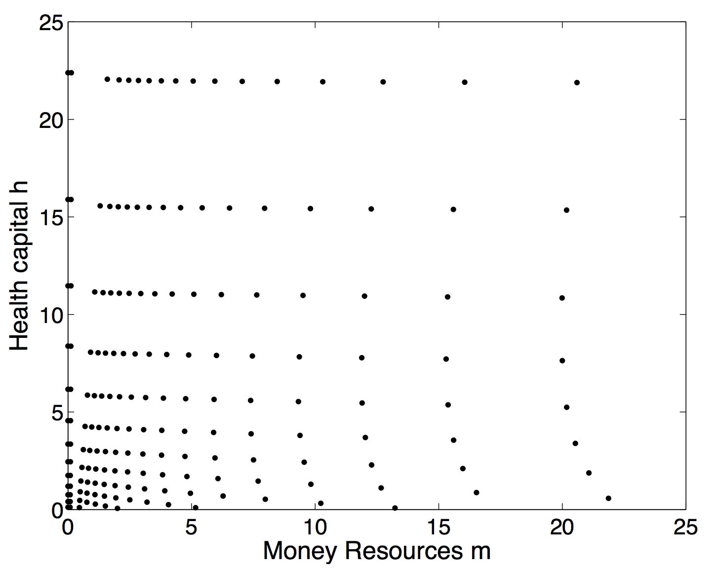
An endogenous grid in a two-dimensional model where the points come from a rectangular grid on the post-decision
states. — An endogenous grid in a two-dimensional model where the points come from a rectangular grid on the post-decision states.

The literature suggests several remedies:

Paper	Suggested remedy
Barillas & Fernández-Villaverde (2007)	avoid the irregular grid: EGM in one choice, value function iterations in the others
Brumm & Grill (2014)	Delaunay triangulation of the endogenous points, linear interpolation within each triangle
Ludwig & Schön (2018)	Delaunay interpolation and hybrid methods compared; the cost of the triangulation can offset the speed of EGM
White (2015)	use the index structure inherited from the rectangular grid: locate the cell by a visibility walk, map it to the unit square, interpolate multilinearly
Druedahl & Jørgensen (2017)	re-interpolate on a regular grid while performing the upper envelope step
Lujan (2026)	interpolate in the index coordinates of the endogenous grid, with no triangulation

Why is locating the cell trivial on a rectangular grid, and what is its cost on an irregular one with $n$ points?
Which of the approaches still works if the endogenous points cross each other, so that neighboring cells overlap?

Several continuous choices without rootfinding: multidimensional EGM¶

A model of wealth and health, or of liquid and illiquid assets, has several continuous states and several continuous choices. EGM carries over without root finding when the problem is triangular Iskhakov, 2015Iskhakov, 2017: the Euler equations can be solved one at a time, each by an analytical inversion.

Take a triangular example in $\mathbb{R}^3$ :

V_t(M_t)=\max_{c}\Big[u(c)+\beta\, \mathbb{E}\big\{V_{t+1}(M_{t+1})\,\big|\,M_t,c\big\}\Big]

$M_t \in \mathbb{R}^3$ is the vector of resources at time $t$
$c_t \in \mathbb{R}^3$ is the utilization of resources
$A_t \in \mathbb{R}^3$ are the resources at the end of $t$ , the post-decision states
$A_t = g(M_t, c_t)$ is the intra-temporal evolution
$M_{t+1} = f(A_t, \tilde R)$ is the inter-temporal evolution, the budget constraint
$\tilde R$ are idiosyncratic stochastic shocks
$u: \mathbb{R}^3 \to \mathbb{R}$ is the utility of current resource utilization

The plan: apply the EGM ideas to discover the necessary assumptions on the fundamentals of the problem that make it possible, abstracting away from the budget constraint and other feasibility restrictions.

Post-decision states¶

We have already assumed that

M_{t+1} = f\big(A_t, \tilde R\big) = f\big(g(M_t, c_t), \tilde R\big),

which allows replacing the condition in the expectation in the Bellman equation:

\mathbb{E}\big\{V_{t+1}(M_{t+1})\,\big|\,M_t, c_t\big\} = \mathbb{E}\big\{V_{t+1}(M_{t+1})\,\big|\,A_t\big\}

The post-decision states $A_t$ are sufficient statistics for $(M_t, c_t)$ .

The corrigendum Iskhakov, 2017 completes the condition: the partial derivatives of $g$ with respect to the choices must depend on the period $t$ variables only through the post-decision states, so that the Euler equations below can be evaluated at a point of the grid on $A_t$ .

Bellman optimization, first order and envelope conditions¶

With the inter-temporal evolution written out by component, the Bellman equation is

V_t(M_t)= \max_{c}\left[u(c)+\beta\, \mathbb{E} \left\{\left.V_{t+1}\begin{pmatrix} f^1(A_t^1,A_t^2,A_t^3,\tilde{R})\\ f^2(A_t^1,A_t^2,A_t^3,\tilde{R})\\ f^3(A_t^1,A_t^2,A_t^3,\tilde{R}) \end{pmatrix}\right|A_t\right\}\right]

The first order conditions are

\begin{aligned} u'_1(c) + \beta\, \mathbb{E} \sum_{i=1}^3 \sum_{j=1}^3 (V_{t+1})'_i\, (f^i)'_j\, (\partial g^j/\partial c^1) &= 0\\ u'_2(c) + \beta\, \mathbb{E} \sum_{i=1}^3 \sum_{j=2}^3 (V_{t+1})'_i\, (f^i)'_j\, (\partial g^j/\partial c^2) &= 0\\ u'_3(c) + \beta\, \mathbb{E} \sum_{i=1}^3 (V_{t+1})'_i\, (f^i)'_3\, (\partial g^3/\partial c^3) &= 0 \end{aligned}

and the envelope conditions are

\begin{aligned} (V_t)'_1 &= \beta\, \mathbb{E} \sum_{i=1}^3 \sum_{j=1}^3 (V_{t+1})'_i\, (f^i)'_j\, (\partial g^j/\partial M_t^1)\\ (V_t)'_2 &= \beta\, \mathbb{E} \sum_{i=1}^3 \sum_{j=2}^3 (V_{t+1})'_i\, (f^i)'_j\, (\partial g^j/\partial M_t^2)\\ (V_t)'_3 &= \beta\, \mathbb{E} \sum_{i=1}^3 (V_{t+1})'_i\, (f^i)'_3\, (\partial g^3/\partial M_t^3) \end{aligned}

Combining these with the first order conditions, we have

\begin{aligned} u'_3(c_t) &= - \frac{\partial g^3/\partial c^3}{\partial g^3/\partial M_t^3}\, (V_t)'_3\\ u'_2(c_t) - u'_3(c_t) &= - \frac{\partial g^2/\partial c^2}{\partial g^2/\partial M_t^2} \Big[(V_t)'_2 - (V_t)'_3\Big]\\ u'_1(c_t) - u'_2(c_t) &= - \frac{\partial g^1/\partial c^1}{\partial g^1/\partial M_t^1} \Big[(V_t)'_1 - (V_t)'_2\Big] \end{aligned}

The system of Euler equations¶

The partial derivatives of the value function $(V_t)'_i$ are now expressed as linear functions of the marginal utilities $\mathcal{L}_{t}[u'(c_t)]$ , with coefficients given by the partial derivatives of the functions $g^i(\bullet)$ . In period $t+1$ they give the system of Euler equations

\begin{aligned} u'_1(c_t^1,c_t^2,c_t^3) &= \beta\, \mathbb{E} \sum_{i=1}^3 \sum_{j=1}^3 \mathcal{L}_{t+1}[u'(c_{t+1})]\, (f^i)'_j\, (\partial g^j/\partial c^1)\\ u'_2(c_t^1,c_t^2,c_t^3) &= \beta\, \mathbb{E} \sum_{i=1}^3 \sum_{j=2}^3 \mathcal{L}_{t+1}[u'(c_{t+1})]\, (f^i)'_j\, (\partial g^j/\partial c^2)\\ u'_3(c_t^1,c_t^2,c_t^3) &= \beta\, \mathbb{E} \sum_{i=1}^3 \mathcal{L}_{t+1}[u'(c_{t+1})]\, (f^i)'_3\, (\partial g^3/\partial c^3) \end{aligned}

$c_{t+1}(M_{t+1})$ is interpolated from the previous iteration of backward induction
the right-hand side is then known, and we need to solve for $c_t^1, c_t^2, c_t^3$

Sufficient conditions for EGM to be applicable¶

The proof is constructive: follow the EGM step for a grid imposed over the post-decision state space.

Algorithm (multidimensional EGM)

Input: a grid of points $A_j = (A^1_j, A^2_j, A^3_j)$ , $j = 1, \dots, n$ , on the post-decision states, quadrature nodes and weights $(\tilde R_k, \omega_k)$ , $k = 1, \dots, K$ , for the shocks, and the terminal policy $c_T(M)$ .

Iterate backward for $t = T-1, T-2, \dots$ :

For every grid point $A_j$ , $j = 1, \dots, n$ :
1. next period resources: $M_{t+1, jk} = f(A_j, \tilde R_k)$ for every quadrature node $k$
2. next period choices: $c_{t+1, jk} = c_{t+1}(M_{t+1, jk})$ , interpolated on the endogenous grid of period $t+1$
3. the right-hand sides of the three Euler equations, by quadrature over $k$
4. back substitution: $c^1_{t,j}$ , $c^2_{t,j}$ , $c^3_{t,j}$ one at a time, each by inverting a marginal utility (TRI2, CON)
5. the endogenous grid point: $M_{t,j}$ from $A_j = g(M_{t,j}, c_{t,j})$ , one component at a time (INV)
The points $(M_{t,j}, c_{t,j})$ , $j = 1, \dots, n$ , give the policy $c_t(M)$ on an endogenous grid.

Output: the policy functions $c_t(M)$ for all periods $t$ .

None of the steps searches. What remains costly is what the method does not remove:

the curse of dimensionality: the grid on $A$ has $n^3$ points, and the expectation in step 3 is an integral over all shocks
interpolation on an irregular grid in step 2: the endogenous points $M_t$ form a grid that is not rectangular, as the example below shows

Interpolation and other multidimensional generalizations¶

The irregular endogenous grid, and the conditions under which the Euler system can be inverted at all, are what the literature on multidimensional EGM works on:

Paper	Idea
Barillas & Fernández-Villaverde (2007)	EGM in one choice, value function iterations in the rest
Hintermaier & Koeniger (2010)	occasionally binding constraints among several endogenous states, via Kuhn–Tucker conditions
Brumm & Grill (2014), Ludwig & Schön (2018)	Delaunay triangulation for interpolation on the irregular grid; its cost can offset the speed of EGM
White (2015)	general theory, an invertibility condition, and interpolation that uses the order of the endogenous points
Iskhakov (2015)	the class of triangular problems solvable without root finding
Druedahl & Jørgensen (2017)	non-convexities and constraints, re-interpolating on a regular grid during an upper envelope step
Lujan (2026)	a choice in several dimensions as a sequence of one-dimensional choices
Hallengreen et al. (2024)	EGM when the inverse marginal utility has no closed form

Two of these ideas are worth seeing in detail.

Choices in sequence. Split the period into a sequence of choices, each with its own pre-decision state $M^i$ and post-decision state $A^i = g^i(M^i, c^i)$ , chained by $M^{i+1} = A^i$ , with the shocks realized only between periods:
$\overset{\tilde\xi}{\longrightarrow} \underbrace{c^1 \rightarrow c^2 \rightarrow c^3}_{\text{period } t} \overset{\tilde\xi}{\longrightarrow} \underbrace{c^1 \rightarrow c^2 \rightarrow c^3}_{\text{period } t+1} \overset{\tilde\xi}{\longrightarrow}$
Each post-decision state then depends only on the earlier choices, which is the triangular structure of TRI1, and each step is a one-dimensional EGM Lujan, 2026.
No analytical inverse. Precompute the marginal utility on a fixed grid, interpolate it, and invert the interpolant numerically. The rest of the EGM step is unchanged, and the method stays an order of magnitude faster than the traditional ones Hallengreen et al., 2024.

Which conditions of the definition of a triangular problem does the sequential formulation satisfy by construction?
Which is cheaper in two dimensions: Delaunay triangulation of the endogenous grid, or a root finder in every point of a regular grid?

References and additional resources

📖 Carroll (2006) “The method of endogenous gridpoints for solving dynamic stochastic optimization problems”
📖 Carroll & Kimball (1996) “On the concavity of the consumption function” — under uncertainty the consumption function is linear only in special cases, such as CRRA utility with return risk and no labor income, as in the Phelps model
📖 Iskhakov et al. (2017) “The endogenous grid method for discrete-continuous dynamic choice models with (or without) taste shocks”
📖 Fella (2014) “A Generalized Endogenous Grid Method for Non-Smooth and Non-Concave Problems”
📖 Druedahl & Jørgensen (2017) “A general endogenous grid method for multi-dimensional models with non-convexities and constraints”
📖 Barillas & Fernández-Villaverde (2007) “A Generalization of the Endogenous Grid Method”
📖 White (2015) “The Method of Endogenous Gridpoints in Theory and Practice”
📖 Ludwig & Schön (2018) “Endogenous Grids in Higher Dimensions: Delaunay Interpolation and Hybrid Methods”
📖 Iskhakov (2015) “Multidimensional endogenous gridpoint method: Solving triangular dynamic stochastic optimization problems without root-finding operations”, and the corrigendum Iskhakov (2017)
📖 Hintermaier & Koeniger (2010) “The method of endogenous gridpoints with occasionally binding constraints among endogenous variables”
📖 Brumm & Grill (2014) “Computing equilibria in dynamic models with occasionally binding constraints”
📖 Lujan (2026) “The Sequential Endogenous Grid Method”
📖 Hallengreen et al. (2024) “The endogenous grid method without analytical inverse marginal utility”
📺 Foundations of Computational Economics, lectures 41–42 fedor.iskh.me/compecon

References¶

Carroll, C. D. (2006). The method of endogenous gridpoints for solving dynamic stochastic optimization problems. Economics Letters, 91(3), 312–320. 10.1016/j.econlet.2005.09.013
Phelps, E. S. (1962). The accumulation of risky capital: A sequential utility analysis. Econometrica, 30(4), 729–743. 10.2307/1909322
Hakansson, N. H. (1970). Optimal investment and consumption strategies under risk for a class of utility functions. Econometrica, 38(5), 587–607. 10.2307/1912196
Carroll, C. D., & Kimball, M. S. (1996). On the concavity of the consumption function. Econometrica, 64(4), 981–992. 10.2307/2171853
Deaton, A. (1991). Saving and Liquidity Constraints. Econometrica, 59(5), 1221–1248. 10.2307/2938366
White, M. N. (2015). The method of endogenous gridpoints in theory and practice. Journal of Economic Dynamics and Control, 60, 26–41. 10.1016/j.jedc.2015.08.001
Druedahl, J., & Jørgensen, T. H. (2017). A general endogenous grid method for multi-dimensional models with non-convexities and constraints. Journal of Economic Dynamics and Control, 74, 87–107. 10.1016/j.jedc.2016.11.005
Iskhakov, F. (2015). Multidimensional endogenous gridpoint method: Solving triangular dynamic stochastic optimization problems without root-finding operations. Economics Letters, 135, 72–76. 10.1016/j.econlet.2015.07.033
Fella, G. (2014). A generalized endogenous grid method for non-smooth and non-concave problems. Review of Economic Dynamics, 17(2), 329–344. 10.1016/j.red.2013.07.001
Iskhakov, F., Jørgensen, T., Rust, J., & Schjerning, B. (2017). The endogenous grid method for discrete-continuous dynamic choice models with (or without) taste shocks. Quantitative Economics, 8(2), 317–365. https://doi.org/10.3982/QE643
Barillas, F., & Fernández-Villaverde, J. (2007). A generalization of the endogenous grid method. Journal of Economic Dynamics and Control, 31(8), 2698–2712. 10.1016/j.jedc.2006.08.005
Brumm, J., & Grill, M. (2014). Computing equilibria in dynamic models with occasionally binding constraints. Journal of Economic Dynamics and Control, 38, 142–160. 10.1016/j.jedc.2013.09.007
Ludwig, A., & Schön, M. (2018). Endogenous Grids in Higher Dimensions: Delaunay Interpolation and Hybrid Methods. Computational Economics, 51(3), 463–492. 10.1007/s10614-016-9611-2
Lujan, A. (2026). The Sequential Endogenous Grid Method. Journal of Economic Dynamics and Control, 105442. 10.1016/j.jedc.2026.105442
Iskhakov, F. (2017). Corrigendum to “Multidimensional endogenous gridpoint method: Solving triangular dynamic stochastic optimization problems without root-finding operations” [Econom. Lett. 135 (2015) 72–76]. Economics Letters, 150, 26. 10.1016/j.econlet.2016.11.002