📖 Dynamic programming

Dynamic programming is the recursive way of writing a sequential decision problem, and every model later in the course is a variation on it: the Bellman equation, the classification of DP models, and one inventory model solved by backwards induction.

cd sb-dse-code
git reset --hard HEAD
git pull

git pull upstream main                                     # collect the task
cp -r tasks/epsilon_inventory solutions/epsilon_inventory  # work on the copy

What is dynamic programming?¶

“DP is recursive method for solving sequential decision problems”

📖 Rust 2006, New Palgrave Dictionary of Economics

In computer science the meaning of the term is broader: DP is a general algorithm design technique for solving problems with overlapping sub-problems.

Dynamic programming in economics¶

DP provides a framework to study decision making over time and under uncertainty and can accommodate learning, strategic interactions between agents (game theory) and market interactions (equilibrium theory)

Many important problems and economic models are analyzed and solved using dynamic programming:

• Dynamic models of labor supply

• Job search

• Human capital accumulation

• Health process, insurance and long term care

• Consumption/savings choices

• Durable consumption

• Growth models

• Heterogeneous agents models

• Overlapping generation models

Dynamic discrete choice (DDC)¶

Extend the discrete choice framework to repeated discrete choice over time

• Given state $s_t \in S$ an agent takes a decision $d_t \in D(s)$ that determines current utility $u_t(s_t,d_t)$ as well as the future states of the world.

• The agent forms (subjective) beliefs about the uncertain next period’s state $s_{t+1}$ that evolve according to a Markov transition probability $p(s_{t+1}|s_t, d_t)$.

• The agent’s problem is to choose a optimal decision rule $\mathbf{\delta} = \{\delta_0,...,\delta_T\}$, where $d_t=\delta_t(s_t)$, that solves

where $\mathbb{E}_{\delta}$ denotes expectation with respect to the controlled stochastic process $\{s_t,d_t\}$ induced by the decision rule $\delta$.

• The difficulty is that we are looking for a set of functions $\mathbf{\delta} = \{\delta_0,...,\delta_T\}$, not just for a set of numbers $\mathbf{d} = \{d_0,...,d_T\}$

• DP simplifies the DDC problem, allowing us to find $\mathbf{\delta} = \{\delta_0,...,\delta_T\}$ using a recursive procedure.

Bellman’s Principle of Optimality¶

An optimal policy has a property that whatever the initial state and initial decision are, the remaining decisions must constitute an optimal policy with regard to the state resulting from the first decision.

📖 Bellman, 1957 “Dynamic Programming”

Breaking the problem into sequence of small problems¶

• Thus, the sequential decision problem is broken into initial decision problem and the future decisions problem

• The solution can be computed through backward induction, i.e. solving a sequential decision problem from the later periods

• Embodiment of the recursive way of modeling sequential decisions is Bellman equation

Bellman equation¶

• State variables — vector of variables that describe all relevant information about the modeled decision process, $x_t$

• Decision variables — vector of variables describing the choices, $d_t$

• Instantaneous payoff — utility function, $u(x_t,d_t)$, with time separable discounted utility

• (next state) is the stochastic next period state resulting from current state and decision

• expectation $\mathbb{E}\{\cdot\}$ is taken over the distribution of the next period state conditional on current state and decision

• Motion rules — agent’s beliefs of how state variable evolve through time, conditional on choices, $x_{t+1} \sim F(x_t,d_t)$

• $\beta$ is a discount factor to measure future rewards in terms of current ones

Solution is given by:

• Value function — maximum attainable utility $V(x_t)$

• Policy function — mapping from state space to action space that returns the optimal choice, $d^{\star}(x_t)$

The optimal choices are revealed along the solution of the Bellman equation as decisions which solve the maximization problem in the right hand side ($\arg\max$ of the maximization in the Bellman equation)

Classification of DP models¶

There are many problems where DP methods are applicable, therefore it is important to quickly classify your problem to make others understand exactly what follows

Whether time is continuous or discrete¶

1. Discrete time

   • time periods $t$, $t+1$

   • dynamics given by difference equations

2. Continuous time

   • all entities in the model are functions of time

   • dynamics given by differential equation

   • so, math is very different

   • continuous time for cleaner theoretical models, sometimes also solved numerically

   • not part of this course

3. Continuous time with discrete events

   • continuous time dynamics, but discrete events (e.g. Poisson process) that change the state of the system

   • appropriate in many settings such as search

   • significant simplification is certain settings

   • 📖 DSE2024 lecture by Peter Arcidiacono on the topic

   • also not part of this course

Whether horizon is finite or infinite¶

1. Finite horizon

   • there is terminal period $T$

   • special form of Bellman equation in period $T$

   • in other words, as if $V(\text{at } T +1 ) = \mathbb{0}$

   • value function and policy function are time dependent

   • solved by backwards induction with $T$ number of steps

2. Infinite horizon

   • time subscripts are dropped, primes for next period values instead

   • solution is given by fixed point of the Bellman operator

   • have to actually solve a functional equation

Most problems can be specified and solved in both finite or infinite horizon

Whether choice space is discrete, continuous, mixed discrete-continuous or discretized¶

1. Problems with discrete choice

   • Rust model of bus engine replacement next week

   • Inventory management of discrete goods (later today)

   • Thousands other problems

   • 📖 Aguirregabiria & Mira (2010) “Dynamic discrete choice structural models: A survey”

2. Problems with continuous choice

   • cake eating and consumption-savings models (later in the course)

   • discretized?

   • treated as continuous?

   • require interpolating of value function in Bellman equation!

   • 📖 Carroll (2006) EGM paper, and Iskhakov (2015) multidimensional EGM paper

3. Problems with discrete and continuous choice

   • much more complicated: kinks in value functions, discontinuous policy function

   • require global optimization in Bellman equation which is not easy

   • one way out is to discretize choices at the cost of reduced accuracy

   • 📖 Iskhakov et al. (2017) DCEGM paper

What about state space?¶

• When choice is discrete, typically state space is also finite

• Even when state variables are continuous, by discretization it is converted to discrete

1. This is true in general when using numerical solvers: state space is discretized within some reasonable bounds

   • choice of upper bounds, number and placement of grid points influence the (accuracy of the) solution

2. Another approach to represent state space is to project value and/or policy function onto space of orthogonal polynomials (Chebyshev polynomials in particular)

   • only works well when value function is sufficiently smooth

Whether model includes stochastic processes¶

1. Deterministic models

   • No random elements, all motion rules deterministic

   • No need for expectation operator in Bellman equation

2. Stochastic models with idiosyncratic shocks

   • expectation does not have to be conditioned on current period shocks

   • which opens a cheaper way of writing the fixed point, and we use it on Thursday

3. General form stochastic models

   • expectation in Bellman equation has to be computed with quadrature or Monte Carlo integration

Whether choice is part of the problem at all¶

• Some problems solved by the DP methods do not have explicit choices and maximization

Example: Inventory management model¶

Consider the following problem in discrete time and finite horizon $t=0,\dots,T$

The notation is:

• $x_t\ge 0$ is inventory at period $t$ measured in discrete units

• $d_t\ge 0$ is potentially stochastic demand at period $t$

• $q_t\ge 0$ is the order of new inventory

• $p$ is the profit per one unit of (supplied) good

• $c$ is the fixed cost of ordering any amount of new inventory

• $r$ is the cost of storing one unit of good

The sales in period $t$ are given by $s_t = \min\{x_t,d_t\}$.

Inventory to be stored till next period is given by $k_t = \max\{x_t-d_t,0\} + q_t = x_{t+1}$.

The profit in period $t$ is given by

Assuming all $q_t \ge 0$, let $\sigma = \{q_t\}_{t=1,\dots,T}$ denote a feasible inventory policy.

The expected profit maximizing problem is given by

where $\beta$ is discount factor.

Bellman equation for the problem¶

So, both $x_t$ and $d_t$ are taken into account for the new order to be made, forming the state space.

The expectation in the Bellman equation is taken over the distribution of the next period demand $d_{t+1}$, which we assume is independent of any other variables and across time (idiosyncratic), thus the conditioning on $(x_t,d_t,s_t)$ can be meaningfully dropped.

Expectation can be written as an integral over the distribution of demand $F(d)$, and since inventory is discrete it's natural to assume demand is as well.

The integral then transforms into a sum over the possible value of demand, weighted by their probabilities $pr(d)$

First deterministic demand¶

Let’s focus first on a deterministic case: let $d$ be fixed and constant over time. How does the Bellman equation change?

In the deterministic case with fixed $d$, it can be simply dropped from the state space, and the Bellman equation can be simplified to

import numpy as np
import matplotlib.pyplot as plt
%matplotlib inline
plt.rcParams['figure.figsize'] = [12, 8]

class inventory_model:
    '''Small class to hold model fundamentals and its solution'''

    def __init__(self,label='noname',
                 max_inventory=10,  # upper bound on the state space
                 c = 3.2,           # fixed cost of order
                 p = 2.5,           # profit per unit of good
                 r = 0.5,           # storage cost per unit of good
                 β = 0.95,          # discount factor
                 demand = 4         # fixed demand
                 ):
        '''Create model with default parameters'''
        self.label=label # label for the model instance
        self.c, self.p, self.r, self.β = c, p, r, β
        self.demand = demand
        # created dependent attributes (it would be better to have them updated when underlying parameters change)
        self.n = max_inventory+1    # number of inventory levels
        self.upper = max_inventory  # upper boundary on inventory
        self.x = np.arange(self.n)  # all possible values of inventory (state space)

    def __repr__(self):
        '''String representation of the model'''
        return 'Inventory model labeled "{}"\nParamters (c,p,r,β) = ({},{},{},{})\nDemand={}\nUpper bound on inventory {}' \
               .format (self.label,self.c,self.p,self.r,self.β,self.demand,self.upper)

    def sales(self,x,d):
        '''Sales in given period'''
        return np.minimum(x,d)

    def next_x(self,x,d,q):
        '''Inventory to be stored, becomes next period state'''
        return x - self.sales(x,d) + q

    def profit(self,x,d,q):
        '''Profit in given period'''
        return self.p * self.sales(x,d) - self.r * self.next_x(x,d,q) - self.c * (q>0)

model=inventory_model(label='test')
print(model)

q=np.zeros(model.n)
print('Current profits with zero orders\n',model.profit(model.x,model.demand,q))

Inventory model labeled "test"
Paramters (c,p,r,β) = (3.2,2.5,0.5,0.95)
Demand=4
Upper bound on inventory 10
Current profits with zero orders
 [ 0.   2.5  5.   7.5 10.   9.5  9.   8.5  8.   7.5  7. ]

# illustration of broadcasting in the inventory model
q=model.x[:,np.newaxis]  # column vector
print('Current inventory\n',model.x)
print('Current sales\n',model.sales(model.x,model.demand))
print('Current orders\n',q)
print('Next period inventory\n',model.next_x(model.x,model.demand,q))
print('Current profits\n',model.profit(model.x,model.demand,q))

Current inventory
 [ 0  1  2  3  4  5  6  7  8  9 10]
Current sales
 [0 1 2 3 4 4 4 4 4 4 4]
Current orders
 [[ 0]
 [ 1]
 [ 2]
 [ 3]
 [ 4]
 [ 5]
 [ 6]
 [ 7]
 [ 8]
 [ 9]
 [10]]
Next period inventory
 [[ 0  0  0  0  0  1  2  3  4  5  6]
 [ 1  1  1  1  1  2  3  4  5  6  7]
 [ 2  2  2  2  2  3  4  5  6  7  8]
 [ 3  3  3  3  3  4  5  6  7  8  9]
 [ 4  4  4  4  4  5  6  7  8  9 10]
 [ 5  5  5  5  5  6  7  8  9 10 11]
 [ 6  6  6  6  6  7  8  9 10 11 12]
 [ 7  7  7  7  7  8  9 10 11 12 13]
 [ 8  8  8  8  8  9 10 11 12 13 14]
 [ 9  9  9  9  9 10 11 12 13 14 15]
 [10 10 10 10 10 11 12 13 14 15 16]]
Current profits
 [[ 0.   2.5  5.   7.5 10.   9.5  9.   8.5  8.   7.5  7. ]
 [-3.7 -1.2  1.3  3.8  6.3  5.8  5.3  4.8  4.3  3.8  3.3]
 [-4.2 -1.7  0.8  3.3  5.8  5.3  4.8  4.3  3.8  3.3  2.8]
 [-4.7 -2.2  0.3  2.8  5.3  4.8  4.3  3.8  3.3  2.8  2.3]
 [-5.2 -2.7 -0.2  2.3  4.8  4.3  3.8  3.3  2.8  2.3  1.8]
 [-5.7 -3.2 -0.7  1.8  4.3  3.8  3.3  2.8  2.3  1.8  1.3]
 [-6.2 -3.7 -1.2  1.3  3.8  3.3  2.8  2.3  1.8  1.3  0.8]
 [-6.7 -4.2 -1.7  0.8  3.3  2.8  2.3  1.8  1.3  0.8  0.3]
 [-7.2 -4.7 -2.2  0.3  2.8  2.3  1.8  1.3  0.8  0.3 -0.2]
 [-7.7 -5.2 -2.7 -0.2  2.3  1.8  1.3  0.8  0.3 -0.2 -0.7]
 [-8.2 -5.7 -3.2 -0.7  1.8  1.3  0.8  0.3 -0.2 -0.7 -1.2]]

Backwards induction¶

Backwards induction algorithm is used to solve finite horizon models

Solver for the finite horizon dynamic programming problems

1. Start at t=T
1. Solve Bellman equation at t, record optimal choice  
1. Decrease t unless t=1, and return to previous step.  

As result, for all t=1,..,T have found the optimal choice (as a function of state)

First, we need to code up the Bellman equation

def bellman(m,v0):
    '''Bellman equation for inventory model
       Inputs: model object
               next period value function
    '''
    # create the grid of choices (same as x), column-vector
    q = m.x[:,np.newaxis]
    # compute current period profit (relying on numpy broadcasting to get the matrix with choices in rows)
    p = m.profit(m.x,m.demand,q)
    # indexes for next period value with extrapolation using last value
    i = np.minimum(m.next_x(m.x,m.demand,q),m.upper)
    # compute the Bellman maximand
    vm = p + m.β*v0[i]
    # find max and argmax
    v1 = np.amax(vm,axis=0)   # maximum in every column
    q1 = np.argmax(vm,axis=0) # arg-maximum in every column = order volume
    return v1, q1

v = np.zeros(model.n)
for i in range(3):
    v,q = bellman(model,v)
    print('Value =',v,'Policy =',q,sep='\n',end='\n\n')

Value =
[ 0.   2.5  5.   7.5 10.   9.5  9.   8.5  8.   7.5  7. ]
Policy =
[0 0 0 0 0 0 0 0 0 0 0]

Value =
[ 4.3    6.8    9.3   11.8   14.3   14.3   14.3   15.625 17.5   16.525
 15.55 ]
Policy =
[4 4 4 4 4 3 2 0 0 0 0]

Value =
[ 9.425 11.925 14.425 16.925 19.425 19.425 19.425 19.71  21.585 21.085
 20.585]
Policy =
[8 8 8 8 8 7 6 0 0 0 0]

def solver_backwards_induction(m,T=10,verbose=False):
    '''Backwards induction solver for the finite horizon case'''
    # solution is time dependent
    m.value  = np.zeros((m.n,T))
    m.policy = np.zeros((m.n,T))
    # main DP loop (from T to 1)
    for t in range(T,0,-1):
        if verbose:
            print('Time period %d\n'%t)
        j = t-1 # index of value and policy functions for period t
        if t==T:
            # terminal period: ordering zero is optimal
            m.value[:,j] = m.profit(m.x,m.demand,np.zeros(m.n))
            m.policy[:,j] = np.zeros(m.n)
        else:
            # all other periods
            m.value[:,j], m.policy[:,j] = bellman(m,m.value[:,j+1]) # next period to Bellman
        if verbose:
            print(m.value,'\n')
    # return model with updated value and policy functions
    return m

model = inventory_model(label='illustration')
model=solver_backwards_induction(model,T=5,verbose=True)
print('Optimal policy:\n',model.policy)

Time period 5

[[ 0.   0.   0.   0.   0. ]
 [ 0.   0.   0.   0.   2.5]
 [ 0.   0.   0.   0.   5. ]
 [ 0.   0.   0.   0.   7.5]
 [ 0.   0.   0.   0.  10. ]
 [ 0.   0.   0.   0.   9.5]
 [ 0.   0.   0.   0.   9. ]
 [ 0.   0.   0.   0.   8.5]
 [ 0.   0.   0.   0.   8. ]
 [ 0.   0.   0.   0.   7.5]
 [ 0.   0.   0.   0.   7. ]] 

Time period 4

[[ 0.     0.     0.     4.3    0.   ]
 [ 0.     0.     0.     6.8    2.5  ]
 [ 0.     0.     0.     9.3    5.   ]
 [ 0.     0.     0.    11.8    7.5  ]
 [ 0.     0.     0.    14.3   10.   ]
 [ 0.     0.     0.    14.3    9.5  ]
 [ 0.     0.     0.    14.3    9.   ]
 [ 0.     0.     0.    15.625  8.5  ]
 [ 0.     0.     0.    17.5    8.   ]
 [ 0.     0.     0.    16.525  7.5  ]
 [ 0.     0.     0.    15.55   7.   ]] 

Time period 3

[[ 0.     0.     9.425  4.3    0.   ]
 [ 0.     0.    11.925  6.8    2.5  ]
 [ 0.     0.    14.425  9.3    5.   ]
 [ 0.     0.    16.925 11.8    7.5  ]
 [ 0.     0.    19.425 14.3   10.   ]
 [ 0.     0.    19.425 14.3    9.5  ]
 [ 0.     0.    19.425 14.3    9.   ]
 [ 0.     0.    19.71  15.625  8.5  ]
 [ 0.     0.    21.585 17.5    8.   ]
 [ 0.     0.    21.085 16.525  7.5  ]
 [ 0.     0.    20.585 15.55   7.   ]] 

Time period 2

[[ 0.      13.30575  9.425    4.3      0.     ]
 [ 0.      15.80575 11.925    6.8      2.5    ]
 [ 0.      18.30575 14.425    9.3      5.     ]
 [ 0.      20.80575 16.925   11.8      7.5    ]
 [ 0.      23.30575 19.425   14.3     10.     ]
 [ 0.      23.30575 19.425   14.3      9.5    ]
 [ 0.      23.30575 19.425   14.3      9.     ]
 [ 0.      24.57875 19.71    15.625    8.5    ]
 [ 0.      26.45375 21.585   17.5      8.     ]
 [ 0.      25.95375 21.085   16.525    7.5    ]
 [ 0.      25.45375 20.585   15.55     7.     ]] 

Time period 1

[[17.9310625 13.30575    9.425      4.3        0.       ]
 [20.4310625 15.80575   11.925      6.8        2.5      ]
 [22.9310625 18.30575   14.425      9.3        5.       ]
 [25.4310625 20.80575   16.925     11.8        7.5      ]
 [27.9310625 23.30575   19.425     14.3       10.       ]
 [27.9310625 23.30575   19.425     14.3        9.5      ]
 [27.9310625 23.30575   19.425     14.3        9.       ]
 [28.2654625 24.57875   19.71      15.625      8.5      ]
 [30.1404625 26.45375   21.585     17.5        8.       ]
 [29.6404625 25.95375   21.085     16.525      7.5      ]
 [29.1404625 25.45375   20.585     15.55       7.       ]] 

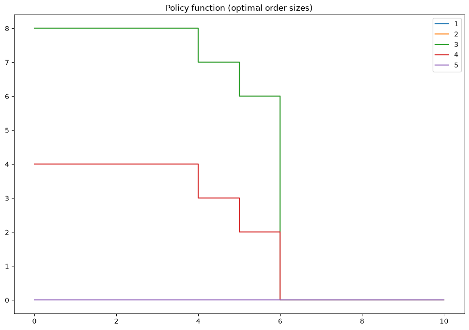
Optimal policy:
 [[8. 8. 8. 4. 0.]
 [8. 8. 8. 4. 0.]
 [8. 8. 8. 4. 0.]
 [8. 8. 8. 4. 0.]
 [8. 8. 8. 4. 0.]
 [7. 7. 7. 3. 0.]
 [6. 6. 6. 2. 0.]
 [0. 0. 0. 0. 0.]
 [0. 0. 0. 0. 0.]
 [0. 0. 0. 0. 0.]
 [0. 0. 0. 0. 0.]]

Source

def plot_solution(model):
    plt.step(model.x,model.value)
    plt.legend([f'{i+1}' for i in range(model.value.shape[1])])
    plt.title('Value function')
    plt.show()
    plt.step(model.x,model.policy)
    plt.legend([f'{i+1}' for i in range(model.policy.shape[1])])
    plt.title('Policy function (optimal order sizes)')
    plt.show()
plot_solution(model)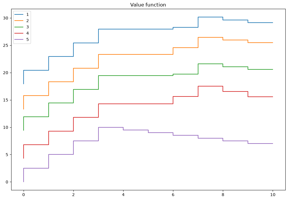

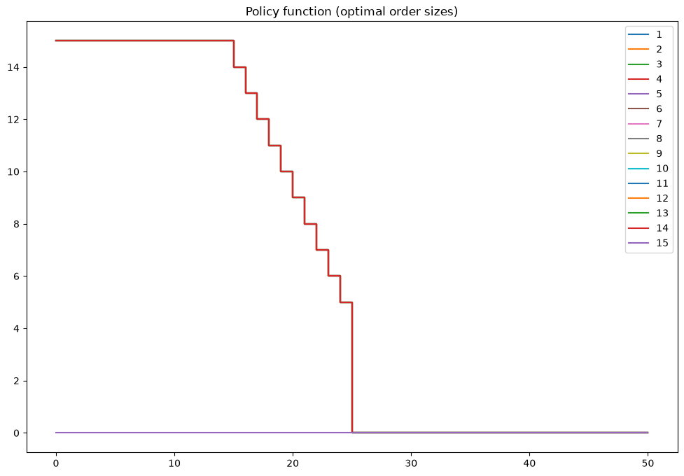
mod = inventory_model(label='production',max_inventory=50)
mod.demand = 15
mod.c = 5
mod.p = 2.5
mod.r = 1.4
mod.β = 0.975
mod = solver_backwards_induction(mod,T=15)
plot_solution(mod)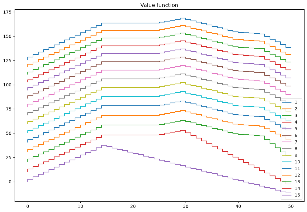

Back to stochastic demand¶

Fixing $d$ was a convenience for the first implementation. Putting the randomness back changes nothing about the method — backwards induction still runs from $T$ down to 1, one Bellman operator per period — and only two things about the code.

The state is a pair. With $d$ random the manager knows the inventory and the realized demand when ordering, so the value function is defined on the grid of $(x,d)$ rather than on $x$ alone, and so is the policy $q^\star(x,d)$.

The Bellman maximand carries an expectation. Next period demand $d'$ is not known when the order is placed, so the continuation value is averaged over it:

with the terminal period unchanged: order nothing, collect the last period’s profit,

A distribution for demand. Take it discrete, on the same grid as the inventory, so that no interpolation is needed anywhere.

Let demand follow a truncated geometric distribution on $\{0,1,\dots,N\}$,

with the last probability corrected so that the vector sums to one — the truncated tail is piled onto $pr_N$. The parameter $\lambda \in (0,1)$ controls how fast demand dies off; the mean of the untruncated distribution is $(1-\lambda)/\lambda$.

Source

N = 25                                    # upper bound of the inventory grid
k = np.arange(N+1)                        # possible values of demand

def demand_pr(lam, n=N+1):
    '''Truncated geometric probabilities over the grid, last one corrected'''
    pr = (1-lam)**np.arange(n) * lam
    pr[-1] = 1 - pr[:-1].sum()            # the truncated tail piles onto the last point
    return pr

rng = np.random.default_rng(2026)
fig, (ax1,ax2) = plt.subplots(1,2,figsize=(12,4))
for lam,clr in [(0.15,'#1A6D91'), (0.25,'#0E8A27'), (0.50,'#CB1515')]:
    pr = demand_pr(lam)
    ax1.step(k, pr, where='mid', color=clr, lw=2,
             label=f'$\\lambda$={lam:.2f}, mean {np.dot(k,pr):.1f}, $pr_N$={pr[-1]:.3f}')
ax1.set_title('Truncated geometric demand')
ax1.set_xlabel('demand $d$'); ax1.set_ylabel('probability')
ax1.legend(frameon=False); ax1.grid(alpha=.3)

lam, T = 0.25, 40
pr = demand_pr(lam)
d = rng.choice(k, size=T, p=pr)           # one path of realized demand
ax2.step(np.arange(T), d, where='mid', color='#0E8A27', lw=1.5)
ax2.axhline(np.dot(k,pr), color='k', ls='--', lw=1, label='mean demand')
ax2.set_title(f'One realization over {T} periods, $\\lambda$={lam:.2f}')
ax2.set_xlabel('period $t$'); ax2.set_ylabel('demand $d_t$')
ax2.legend(frameon=False); ax2.grid(alpha=.3)
plt.show()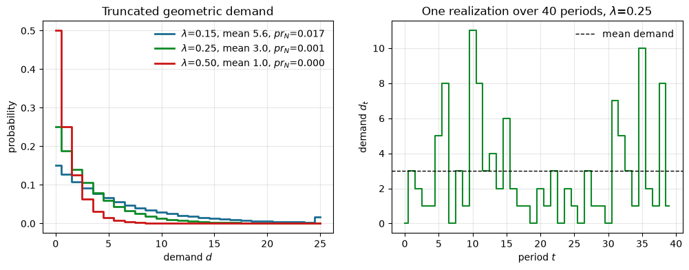

Two things to read off the left panel. The distribution is decreasing, so on this specification small demands are the likely ones, and $\lambda$ moves the mean without changing that shape. And the mass sitting on the last grid point is the truncation: at $\lambda=0.15$ it is 0.017, small but not nothing, which is the price of capping demand at the top of the inventory grid. If a run of the model ever leans on that point, the grid is too short.

The right panel is what the manager actually faces — one path of realized demand. There is no smoothness to exploit and no trend to extrapolate: each period is an independent draw, which is exactly the assumption that lets us write the expectation as a sum with fixed weights.

Origin of the term Dynamic Programming¶