🔬 Practice: Zurcher estimated with CCP

Today we code the two-step CCP estimator of Class 12 for the Zurcher model and put it next to the NFXP estimator of Class 10. Finite dependence turns the dynamic model into a static logit that takes milliseconds to estimate. The price is paid in the first stage, and we will see exactly where.

cd sb-dse-code
git reset --hard HEAD
git pull

One-period finite dependence in the Zurcher model¶

Engine replacement is a renewal action. After a replacement at $t+1$, the mileage at $t+2$ is drawn from $\pi(\cdot|0)$ independent of what happened at $t$. So the two choice sequences keep, then replace and replace, then replace reach the same distribution of the state after one period. Take $d=\text{keep}$, $d'=\text{replace}$ and the renewal action $r=\text{replace}$, and use the EV1 mapping $\psi(x',\text{replace}) = \gamma - \log P(\text{replace}|x')$:

Neither $u(x',\text{replace}) = -RC$ nor $\gamma$ depends on $x'$. Both multiply the difference of two probability distributions, each integrates to one giving difference of zero, so they drop out:

Writing the future relative to keep instead does not work: $v(x+1,\text{keep}) \ne v(0,\text{keep})$, so nothing cancels.

Section 2 of Arcidiacono & Miller (2011) work with a modified Zurcher model where transition probabilities and costs are specified differently. With their deterministic increment of one mileage unit and a reset to zero, the sum collapses to $\beta \log P(\text{replace}|0) - \beta \log P(\text{replace}|x+1)$.

In the parameterization of zurcher.py, $u(x,\text{keep}) = -0.001\,c\,x$ and $u(x,\text{replace}) = -RC$, and replacing moves the bus by the first row of the keep transition matrix $\Pi$. The choice probability becomes

where $\Lambda(\bullet) = \exp(\bullet)/[1+\exp(\bullet)]$ converts value difference to choice probability.

CCP estimator¶

Stage 1

Using data pairs $(x_t,d_t)$ over a panel with at least two periods:

• estimate CCP $P(\text{replace}|x)$ for each $x$

• estimate transition probabilities $\Pi_{x,x'}$ when the engine is kept for each $x$ and $x'$

using consistent estimator, e.g. the frequency estimator or a flexible logit model

Stage 2

Form a (pseudo) statistical criterion as a function of first stage estimates and the structural parameters $(RC, c)$, and apply standard estimation technique, for example GMM, MSM or MLE.

In our case we have $P(\text{keep}|x)$ as a function of $(RC, c)$ and the first-stage CCPs, so we can use MLE in a standard static binary logit with a given offset.

There is no fixed point to solve, not once!

The NFXP benchmark and the offset¶

The representation is exact, not an approximation. Here we need the NFXP estimates as the benchmark to compare with, and the model’s own CCPs at those estimates for the plots below.

import sys, pathlib, tempfile, urllib.request
CODE = pathlib.Path('../gh-code/session10-11')       # the NFXP code of Classes 10-11
if not CODE.exists():                                 # otherwise fetch it from the code repository
    CODE = pathlib.Path(tempfile.mkdtemp())
    url = 'https://raw.githubusercontent.com/fediskhakov/sb-dse-code/main/session10-11/'
    for f in ('zurcher.py', 'nfxp.py', 'busdata1234.csv'):
        urllib.request.urlretrieve(url + f, CODE / f)
sys.path.insert(0, str(CODE))

import numpy as np
import matplotlib.pyplot as plt
from numpy.polynomial import chebyshev
from nfxp import read_busdata, estim_zurcher

data = read_busdata()                        # bus groups 1-4, 175 bins, 450 000 miles
est = estim_zurcher(data)                    # the model with the data attached
res = est.estimate(full=False)               # NFXP partial likelihood: (RC, c), p fixed
print(res)

ev, pk, _ = est.solve()                      # the model at the NFXP estimates
_, v_rep, L = est.choice_values(ev)
logP_rep = v_rep - L                         # log P(replace|x) as a difference, never log of a probability

NFXP estimates, beta = 0.9999, n = 175, N = 8156 bus-months
method bhhh, converged True, 0.438 s, 52 inner solves, 183 inner iterations
parameter     estimate        s.e.
RC             9.76863     1.22592
c              1.34286     0.31520
log-likelihood -8607.8894

def fd_offset(model, logP_rep):
    '''Future term of v(x,keep) - v(x,replace) under one-period finite dependence:
    -beta * sum_x' log P(replace|x') [pi(x'|x,keep) - pi(x'|x,replace)]'''
    Pi = model.trpr                                  # keep: row x of the transition matrix
    return -model.beta * (Pi - Pi[0]) @ logP_rep     # replace: row 0, a fresh engine, for every x

Pi - Pi[0] broadcasts: row 0 is subtracted from every row, so the whole offset is one matrix-vector product. The code omits $\gamma$ from the logsum throughout, which is harmless because it cancels.

First stage: CCPs from the data¶

The two-step estimator replaces the model’s CCPs by estimates from the data, and the transition matrix by the increment frequencies that estim_zurcher already computes in its stage 1. The algorithm:

Input: panel (x_it, d_it), transition matrix Π estimated from increment frequencies
Algorithm:
  1. Estimate log P(replace|x) on the whole mileage grid
  2. offset(x) = -β Σ_x' log P(replace|x') [Π(x,x') - Π(0,x')] for every grid point
  3. Maximize the logit likelihood of keep with index RC - 0.001 c x + offset(x)
Output: estimates of (RC, c), without solving the model

The natural first stage is the bin estimator, replacements over visits in each mileage bin:

def ccp_frequency(model):
    '''Bin estimator of P(replace|x): replacements over visits, NaN where never visited'''
    visits = np.bincount(model.x, minlength=model.n)
    replacements = np.bincount(model.x, weights=model.d, minlength=model.n)
    with np.errstate(invalid='ignore'):              # 0/0 in the unvisited bins
        return replacements / visits, visits

P_freq, visits = ccp_frequency(est)
print(f'{(visits == 0).sum()} of {est.n} bins never visited, '
      f'{((visits > 0) & (P_freq == 0)).sum()} visited but no replacement observed')
with np.errstate(divide='ignore'):
    offset = fd_offset(est, np.log(P_freq))
print(f'finite offsets: {np.isfinite(offset).sum()} of {est.n}')

24 of 175 bins never visited, 105 visited but no replacement observed
finite offsets: 0 of 175

/tmp/ipykernel_3569/769908632.py:5: RuntimeWarning: invalid value encountered in matmul
  return -model.beta * (Pi - Pi[0]) @ logP_rep     # replace: row 0, a fresh engine, for every x

It fails completely. Zurcher replaced 60 engines in 8156 bus-months, and most mileage bins either were never visited or never saw a replacement. The log of a zero frequency is $-\infty$, and since the offset at every $x$ involves the bins right after a fresh engine, $x' = 0, \dots, J$, where nobody replaces, not a single offset is finite.

The first stage has to be smoothed. A flexible logit of the replacement dummy on a polynomial in mileage is the standard choice: it pools information across bins and extrapolates to the ones with no replacements. We need a logit estimator for the first stage and again for the second, so we write it once:

def logit_mle(X, y, offset=0.0, tol=1e-10, maxiter=100, callback=None):
    '''Binary logit P(y=1|X) = Lambda(X b + offset) by Newton's method with step halving,
    with given tolerance and number of iterations.
    Callback function is invoked at each iteration if given.
    Returns b, standard errors from the inverse Hessian, and the log-likelihood.
    '''
    def loglik(b):
        z = X @ b + offset
        return np.sum(y * z - np.logaddexp(0, z))  # log Lambda(z) = z - log(1 + e^z), no overflow
    b0 = np.zeros(X.shape[1])
    for i in range(maxiter):
        p = 0.5 * (1 + np.tanh((X @ b0 + offset) / 2))  # Lambda(z), stable for any z
        g = X.T @ (y - p)                              # score
        H = (X * (p * (1 - p))[:, None]).T @ X         # minus the Hessian, positive definite
        step = np.linalg.solve(H, g)                   # Newton step
        while loglik(b0 + step) < loglik(b0) and np.abs(step).max() > tol:
            step /= 2                                  # plain Newton overshoots from b = 0
        b1 = b0 + step
        err = np.abs(b1 - b0).max()
        if callback != None: callback(err=err, b0=b0, b1=b1, iter=i)
        if err < tol: break
        b0 = b1
    else:
        raise RuntimeError('Failed to converge in %d iterations' % maxiter)
    return b1, np.sqrt(np.diag(np.linalg.inv(H))), loglik(b1)

The structure is that of newton() in the Classic solvers lecture: tol, maxiter and an optional callback, and a for ... else loop that raises an error if the iterations run out.

The logit likelihood is globally concave, but that does not make plain Newton safe: from $b=0$ the first step on the second-stage problem below lands at $c \approx -230$, the next at $c \approx 120$, and the iterations diverge. Halving the step until the likelihood improves fixes it. The first stage uses Chebyshev polynomials of mileage mapped to $[-1,1]$, because with the plain powers $x^k$ the Hessian of the first stage is numerically singular already at degree 5:

def ccp_logit(model, degree=3, full=False):
    '''Flexible logit first stage: log P(replace|x) on the whole grid from a logit in
    Chebyshev polynomials of mileage, which extrapolates to the bins without replacements.
    With full=True also returns the coefficients, their standard errors and the log-likelihood.'''
    basis = lambda x: chebyshev.chebvander(2 * x / model.n - 1, degree)   # grid mapped to [-1, 1]
    b, se, ll = logit_mle(basis(model.x), model.d)
    logP = -np.logaddexp(0, -basis(model.grid) @ b)       # log Lambda(z) = -log(1 + e^{-z})
    return (logP, b, se, ll) if full else logP

degrees = (1, 2, 3, 4, 5, 10)
first_stage, fits = {}, {}
for degree in degrees:
    logP, b, se, ll = ccp_logit(est, degree, full=True)
    first_stage[degree], fits[degree] = logP, (b, se, ll)

# table: one column per degree, estimates with standard errors in brackets
print(f'{"":<18}' + ''.join(f'{"degree " + str(d):>18}' for d in degrees))
for k in range(max(degrees) + 1):
    cells = [f'{b[k]:.3f} ({se[k]:.3f})' if k < b.size else '' for b, se, _ in fits.values()]
    print(f'{"T" + str(k):<18}' + ''.join(f'{c:>18}' for c in cells))
print(f'{"log-likelihood":<18}' + ''.join(f'{ll:>18.2f}' for _, _, ll in fits.values()))
print(f'{"log P(replace|0)":<18}' + ''.join(f'{first_stage[d][0]:>18.2f}' for d in degrees))

                            degree 1          degree 2          degree 3          degree 4          degree 5         degree 10
T0                    -4.160 (0.131)    -5.752 (0.556)    -5.793 (0.683)    -5.476 (2.361)   -11.701 (5.767) 101.526 (101.267)
T1                     3.152 (0.344)     2.745 (0.483)     7.752 (2.336)     7.626 (2.424)   34.863 (16.502) 407.997 (298.969)
T2                                      -2.017 (0.635)    -2.050 (0.770)    -1.572 (3.504)   -10.589 (8.303) 221.165 (191.744)
T3                                                         2.269 (1.005)     2.219 (1.040)    18.469 (9.448) 260.330 (199.718)
T4                                                                           0.174 (1.250)    -2.715 (2.654) 214.513 (163.634)
T5                                                                                             4.728 (2.566)   98.775 (90.264)
T6                                                                                                           151.201 (111.326)
T7                                                                                                             16.798 (30.153)
T8                                                                                                             66.100 (48.843)
T9                                                                                                              -0.118 (6.598)
T10                                                                                                            13.684 (10.231)
log-likelihood               -306.92           -299.66           -296.70           -296.70           -294.55           -293.37
log P(replace|0)               -7.31            -10.51            -17.86            -16.72            -83.07            -15.59

Second stage: a static logit with an offset¶

With the offset computed from the first stage, the second stage is the logit of logit_mle with two regressors, the constant for $RC$ and $-0.001\,x$ for $c$, and the offset passed through:

def estimate_ccp(model, logP_rep):
    '''Second stage: P(keep|x) = Lambda(RC - 0.001 c x + offset(x)), a static logit in
    (RC, c) with the future term computed from the first-stage CCPs'''
    offset = fd_offset(model, logP_rep)
    X = np.column_stack([np.ones(model.N), -0.001 * model.x])   # coefficients: RC and c
    return logit_mle(X, 1 - model.d, offset[model.x])           # y = 1 for keep

print(f'{"first stage":<16}{"RC":>8}{"s.e.":>8}{"c":>8}{"s.e.":>8}{"loglik":>10}{"-log P(rep|0)":>15}')
print(f'{"NFXP":<16}{res.theta[0]:8.3f}{res.se[0]:8.3f}{res.theta[1]:8.3f}{res.se[1]:8.3f}'
      f'{res.stages[0]["loglik_choice"]:10.2f}{-logP_rep[0]:15.2f}')
for degree, lp in first_stage.items():
    try:
        th, se, ll = estimate_ccp(est, lp)
        print(f'{"logit, degree " + str(degree):<16}{th[0]:8.3f}{se[0]:8.3f}{th[1]:8.3f}{se[1]:8.3f}'
              f'{ll:10.2f}{-lp[0]:15.2f}')
    except np.linalg.LinAlgError:                # predicted probabilities all 0 or 1
        print(f'{"logit, degree " + str(degree):<16}{"fails: singular Hessian":>42}{-lp[0]:15.2f}')

first stage           RC    s.e.       c    s.e.    loglik  -log P(rep|0)
NFXP               9.769   1.226   1.343   0.315   -300.57           9.77
logit, degree 1    7.346   0.374   0.720   3.960   -306.64           7.31
logit, degree 2   10.528   0.505   1.795   5.483   -299.60          10.51

logit, degree 3   17.471   0.499   1.324   5.423   -296.77          17.86
logit, degree 4   16.399   0.499   1.310   5.424   -296.77          16.72
logit, degree 5                    fails: singular Hessian          83.07
logit, degree 10                   fails: singular Hessian          15.59

The estimate of $c$ is fairly stable across the first stages, between 1.3 and 1.8 for degrees 2 to 4, around the NFXP value. The estimate of $RC$ is not: it ranges from 7.3 to 17.5, and it follows the last column almost one for one. The plot of the first stages shows why.

Source

fig, ax = plt.subplots(figsize=(8, 4.5))
miles = est.thousand_miles(est.grid)
ax.plot(miles, logP_rep, 'k', lw=2.5, label='NFXP model')
for degree, lp in first_stage.items():
    ax.plot(miles, lp, lw=1.2, label=f'first-stage logit, degree {degree}')
seen = P_freq > 0
ax.scatter(miles[seen], np.log(P_freq[seen]), s=14, c='gray', label='frequency, where positive')
ax.set(xlabel='mileage since last replacement, thousand miles', ylabel='log P(replace | x)',
       ylim=(-20, 0.5))
ax.legend(loc='lower right')
plt.show()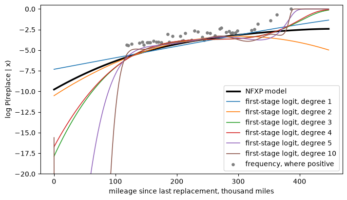

Where replacements are observed, between roughly 120 and 300 thousand miles, all first stages agree with each other and with the model. Below 100 thousand miles there are no replacements at all, and each polynomial extrapolates in its own way, reaching $\log P(\text{replace}|0)$ anywhere from -7 to -18. That is exactly where the offset needs them: $\text{offset}(x)$ contains $\beta \sum_{x'} \Pi_{0,x'} \log P(\text{replace}|x')$, the same constant for every observation, and a constant in the index of a logit is absorbed by the intercept, $RC$. The data identify $RC$ only through the CCPs of a fresh engine, which Zurcher’s data never show being replaced. Push the degree to 5 and the extrapolated $\log P(\text{replace}|0)$ falls below -80; the offsets are then so large that every predicted probability is 0 or 1, and the Hessian of the second stage is singular.

The same second stage with estimagic¶

Writing the Newton iterations by hand shows what happens inside. In practice a package does the optimization and the inference:

• estimagic estimates a model by maximum likelihood given only the log-likelihood contributions, one per observation

• it is installed as part of the package optimagic, the optimization library it was renamed into; import estimagic still provides the estimation functions

• the optimizer is chosen by name, here L-BFGS-B from SciPy

• standard errors come from the outer product of the scores ("jacobian", the default), the Hessian, or the robust sandwich of the two, all by numerical differentiation unless derivatives are supplied

The second version of logit_mle has the same inputs and outputs as the first:

import optimagic as om                         # pip/conda package optimagic, which ships
import estimagic as em                         # estimagic alongside it as a separate module

@om.mark.likelihood                            # tells estimagic these are per-observation contributions
def logit_loglike(params, X, y, offset):
    '''Log-likelihood contribution of every observation of the binary logit'''
    z = X @ params + offset
    return y * z - np.logaddexp(0, z)

def logit_mle_em(X, y, offset=0.0, algorithm='scipy_lbfgsb'):
    '''Binary logit by estimagic: b, standard errors from the Hessian, log-likelihood'''
    res = em.estimate_ml(loglike=logit_loglike, params=np.zeros(X.shape[1]),
                         optimize_options=algorithm,
                         loglike_kwargs=dict(X=X, y=y, offset=offset))
    b = res.params
    return b, res.se(method='hessian'), logit_loglike(b, X, y, offset).sum()

Run both on the second stage with the degree 3 first stage:

offset = fd_offset(est, first_stage[3])
X = np.column_stack([np.ones(est.N), -0.001 * est.x])
for name, fit in (('Newton', logit_mle), ('estimagic', logit_mle_em)):
    th, se, ll = fit(X, 1 - est.d, offset[est.x])
    print(f'{name:<10} RC {th[0]:8.4f} ({se[0]:.4f})  c {th[1]:7.4f} ({se[1]:.4f})  loglik {ll:9.4f}')

Newton     RC  17.4709 (0.4991)  c  1.3238 (5.4234)  loglik -296.7745
estimagic  RC  17.4709 (0.4963)  c  1.3239 (5.3908)  loglik -296.7745

The two agree to the tolerance of the optimizer, about 10^-4 in $c$. The standard errors differ in the second digit, because estimagic differentiates numerically, and they share the same flaw discussed below: both treat the offset as data.

Where it breaks¶

The comparison with NFXP isolates three problems of the two-step approach, none of which shows up in the likelihood value.

• The first stage carries the identification. NFXP pins $RC$ through the model: the CCPs at low mileage are implied by the fitted behavior at high mileage. The two-step estimator takes them from a reduced-form regression that has no information there, and the choice of the smoother, which the theory does not make for us, decides the answer.

• The likelihood does not discipline the first stage. The second-stage log-likelihood of degrees 3 and 4, -296.8, is higher than that of NFXP, -300.6, because nothing forces the first-stage CCPs to be consistent with the estimated structural parameters. Choosing the first stage by the fit of the second is therefore meaningless.

• The standard errors are wrong, in both directions. logit_mle treats the offset as data, so the reported standard error of $RC$, 0.5, ignores all the first-stage uncertainty that the plot displays. The standard error of $c$, 5.4 against 0.3 for NFXP, is a genuine efficiency loss: the future is differenced out, so $c$ is identified from one month of maintenance costs, $-0.001\,c\,x$, while in NFXP it also enters through the discounted stream of all future costs.

What the two-step estimator buys is speed. One CCP estimation takes about 8 ms here, against 0.18 s for the NFXP partial likelihood, and the gap grows with the state space, because the second stage never touches a matrix of the size of the state space beyond one matrix-vector product. Pseudo-likelihood methods, which update the CCPs using the model, are the way to keep the speed and restore the discipline, and they are the subject of Class 14.

Exercises¶

All four start from the objects defined above: data, est, res, logP_rep, P_freq and the functions fd_offset, logit_mle, ccp_logit and estimate_ccp.

Frequency first stage with a floor¶

The bin estimator becomes usable once the zeros are replaced by a small floor $\varepsilon$, and so do the unvisited bins:

for eps in (1e-2, 1e-3, 1e-4, 1e-6):
    lp = np.log(np.clip(np.nan_to_num(P_freq), eps, 1))   # NaN -> 0 -> eps
    th, se, ll = estimate_ccp(est, lp)
    print(f'floor {eps:g}:  RC {th[0]:7.3f}  c {th[1]:7.3f}  loglik {ll:9.2f}')

Monte Carlo: which part of the error comes from the first stage?¶

Simulate panels from the model at the NFXP estimates, using sim_zurcher.py in the folder of this class, and estimate each of them three ways: the infeasible two-step estimator with the true CCPs logP_rep in the first stage, the feasible one with the flexible logit, and NFXP.

from sim_zurcher import simulate

for N in (100, 1000, 10000):                                # buses, 120 months each
    sim = simulate(est, N=N, T=120, seed=1, pk=pk, x0=0)    # new engines at the start, like the data
    m = estim_zurcher(sim, J=est.J, p=est.p)                # same grid and transition probabilities
    th_inf, se_inf, _ = estimate_ccp(m, logP_rep)           # true CCPs
    th_3, _, _ = estimate_ccp(m, ccp_logit(m, 3))           # estimated CCPs
    r = m.estimate(full=False)
    print(f'N {N:6d}  infeasible RC {th_inf[0]:6.3f} c {th_inf[1]:6.3f} (s.e. {se_inf[1]:.2f})  '
          f'logit-3 RC {th_3[0]:6.3f} c {th_3[1]:6.3f}  NFXP RC {r.theta[0]:6.3f} c {r.theta[1]:6.3f} (s.e. {r.se[1]:.2f})')

Estimation under different $\beta$¶

for beta in (0.0, 0.9, 0.99, 0.9999):
    m = estim_zurcher(data, beta=beta)
    th, _, _ = estimate_ccp(m, ccp_logit(m, 3))
    r = m.estimate(full=False)
    print(f'beta {beta:<7} CCP RC {th[0]:8.3f} c {th[1]:7.3f}   NFXP RC {r.theta[0]:8.3f} c {r.theta[1]:7.3f}')

Run time¶

%timeit estimate_ccp(est, ccp_logit(est, 3))
%timeit estim_zurcher(data).estimate(full=False)

Compare the two, then repeat on a grid of twice and four times as many bins, read_busdata(n=350, max_miles=900_000) and so on, and report how each time scales with $n$.